Solutions to the puzzle
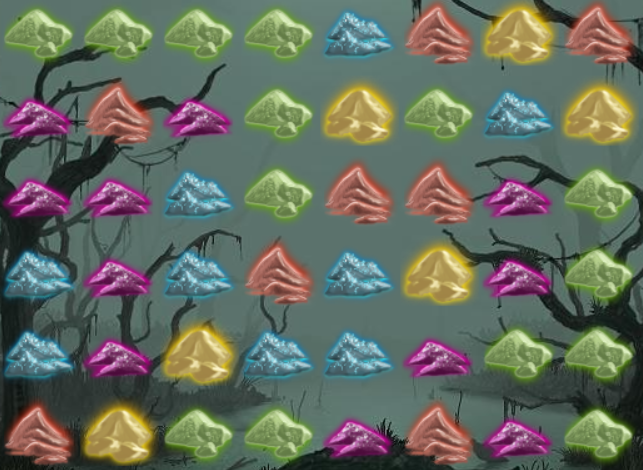
This is (perhaps?) the final post in the series about solving a dust-matching puzzle pictured below, where the whole cluster of similar-colored piles are removed when one in the cluster is clicked, and the piles the fall down and towards the center to fill any voids that are created.
 I wrote a depth first search (DFS) solver that is able to find the best solution, given enough time, and have also written a deep neural network (NN) solver that can be trained to approximate the DFS solutions, to solve puzzles faster.
Both of these methods effectively relied on brute force enumeration of possible results to find a good answer, which is arguably not a very “intelligent” way of approaching a problem.
The benefit here is that an exhaustive brute force search is guaranteed to find the shortest solution, while the downside is that a lot of computation has to go into finding these solutions.
Indeed, the NN solution took several days to train to reliably reproduce the DFS approach, but this was only done for a time-limited DFS approach, which required the DFS solution finder to terminate within 15 seconds, and therefore rarely finding the actual shortest solution.
It could take months (or more!) to produce enough training data for a neural network to reliably find the best solution with this approach.
I wrote a depth first search (DFS) solver that is able to find the best solution, given enough time, and have also written a deep neural network (NN) solver that can be trained to approximate the DFS solutions, to solve puzzles faster.
Both of these methods effectively relied on brute force enumeration of possible results to find a good answer, which is arguably not a very “intelligent” way of approaching a problem.
The benefit here is that an exhaustive brute force search is guaranteed to find the shortest solution, while the downside is that a lot of computation has to go into finding these solutions.
Indeed, the NN solution took several days to train to reliably reproduce the DFS approach, but this was only done for a time-limited DFS approach, which required the DFS solution finder to terminate within 15 seconds, and therefore rarely finding the actual shortest solution.
It could take months (or more!) to produce enough training data for a neural network to reliably find the best solution with this approach.
It’s important to note here that the bottleneck is that both the DFS and NN approach both relied on this brute force method. So, the question becomes: how to create an algorithm that can find the shortest solutions without being shown the shortest solution?
Reinforcement Learning
Machine learning can roughly be broken down into three paradigms:
- Supervised learning, like the NN method referenced above, where the machine is shown correct/tagged input data, and generalizes to other input data.
- Unsupervised learning, where the machine categorizes/encodes untagged input data based on learned correlations within the dataset.
- Reinforcement learning, where the machine “tags” input data subject to some reward function (which need not be a function of the input data or tags), and seeks to maximize that reward.
Reinforcement learning has been demonstrated effective at finding solutions to other games, as AlphaGo demonstrated with the game Go. Indeed, the company DeepMind has applied reinforcement learning to many practical problems, as well as games. This makes reinforcement learning an attractive paradigm for solving this puzzle, while presenting the additional excitement of being the paradigm of machine learning that I have not yet tinkered with.
Framing the puzzle
For games, reinforcement learning is typically framed in the context of an actor which can take actions that results in a reward in an environment that is described by states. The critical parts here are the actions, which correspond to moves or a particular dust pile to click, and states, which are the colors of dust piles in each grid location that are considered before making any particular move. After taking an action, the state of the environment changes, and a reward is received. The reward (a number) should then be defined in such a way that the desired behavior results in the highest reward. How exactly to define the reward is a problem left to any particular application of reinforcement learning.
In a general sense, a positive (or large) reward should be given for “good” or “useful” actions, while a negative (or zero/small) reward given for less ideal actions. There are many different reinforcement learning strategies out there, but ultimately all aim to maximize the reward of actions. In the game scenario, this means not only maximizing the reward of a particular action, but maximizing the reward of the entire chain of actions that make up one complete game. With that in mind, there are several ways one might define the reward of a particular action in the game:
- A reward only for completing a game, to promote solutions that clear the board
- A reward based on the number of piles removed for an action, to prioritize “good moves”
- A penalty (negative reward) for each step in a solution, to prioritize shorter solutions
In practice, some combination of these will likely result in optimal solutions. But how does this optimization happen, and what is optimized?
Quality™
In a very general sense, reinforcement learning will determine a policy for selecting actions given a particular state. This policy will not only take into account the current reward, but also potential future rewards that the actor might receive from the new state resulting from the selected action. Mathematically, this policy can be described as selecting the action with the highest quality for a given state , which is a sum of current and future rewards. If the quality is taken to be a function of the current state and potential actions, then the selected action will be:
Usually potential actions is some small finite set, in which case the argmax, which finds the that produces the maximum is easy to determine. In this case, potential actions are a location to click on the 8 by 6 grid.
This application of reinforcement learning thus boils down to determining the quality function for the chosen reward scheme. As long as the reward incentives the desired behavior, and the quality function accurately reproduces the current and future rewards, choosing actions based on the maximal quality will result in the desired behavior. So the very general and widely applicable question central to reinforcement learning becomes: how does one determine a quality function?
Q-Learning
Q-Learning is one of the most popular reinforcement learning algorithms for determining a quality function. It is based on the Bellman equation which prescribes an iterative approach to determining a quality function. Basically, one starts with a totally random, or zero initialized, quality function and repeats the following procedure to update the quality function:
- Observe a (random) state to determine the best action according to the current quality function, and calculate its reward .
- According to the quality function, find the maximum quality possible for the state generated by the best action .
- Update the quality function such that it is closer to the sum of the reward and the maximum quality of the next state.
Mathematically speaking, the new value for the quality function is given by:
where is a “learning rate” parameter, and is a “discount factor” which determines how important future rewards are to the quality, both bounded by , and selected based on the problem being optimized. If both the learning rate and discount factor are set to 1, as is appropriate for a fully deterministic problem like this puzzle, it is clear that at each step the quality is simply set to the sum of future quality and the current reward. As qualities (rewards) are set for states near the end of the game, these will be iteratively propagated back to early-game states. Eventually, the quality function will converge to the desired behavior, and critically does not require known solutions, opting instead for an exploratory approach to any given problem, and a model of how actions result in state transitions.
In the simplest form, Q-learning represents the quality function as a lookup table for each possible state and action pair, which is guaranteed to work but may be intractable if there are too many possible states or actions. Here there are more than possible states, which is intractable, so approximations must be made.
Deep Q-Learning
The problem now is that there are simply too many sets of possible states and actions to possibly represent in exhaustive detail, and even if it were possible, it would take a very long time to iteratively update such a lookup table to converge to a good quality function. But all is not lost! In the last decade significant advances have been made using neural networks to model quality functions with intractably large state spaces. DeepMind networks have, for instance, used convolutional networks to process the images from Atari video games as input states, and achieved expert-level performance with the resulting quality functions.
The process is essentially the same as standard Q-learning, except that instead of simply updating a value in a lookup table, the Bellman equation update rule is used to generate “true” data for the network to learn, given a particular state as input. So the network is used to predict the quality of an action for a given state, and then trained on the reward and maximum quality of the next state. In this way, the neural network takes the place of an exhaustive lookup table, and learns how to calculate the quality function.
Modeling the quality function
Since the model in my previous post reproduced the results of the DFS solver quite well, I decided to use a very similar topology to model the quality function, which allows me to reuse a lot of code from the previous post. Here, each element in the output tensor will represent the quality of the action that corresponds to clicking that grid location. The primary difference here is that instead of sigmoid output to represent probabilities in the last layer, I have used linear activation (no activation) more appropriate for modeling arbitrary quality values. I have also switched from using binary cross-entropy loss (again, more appropriate for probabilities) to using Huber loss. Huber loss is very close to mean squared error loss, but behaves linearly instead of quadratically for outliers, resulting in better numerical stability (fewer very large numbers in error calculations). Generally speaking mean squared error, or variants like Huber error, are appropriate for regression problems, like modeling a function. I have also reduced the total number of layers from 10 to 5, after some experimentation showed no significant advantage for so many layers. This significantly speeds up training time, particularly early on.
import tensorflow as tf
from tensorflow.keras import Input
from tensorflow.keras.layers import Dense
from tensorflow.keras.models import Model, load_model
from tensorflow.keras.initializers import HeNormal
from tensorflow.keras.losses import Huber

width = 8
height = 6
nsym = 5

board_state = Input(shape=(width,height,nsym+1), name='board_state')
last = Flatten(name='flatten')(board_state)
for i in range(5):
    last = Dense(1500, name='hidden%i'%i, activation='relu', kernel_initializer=HeNormal())(last)
dense = Dense(width*height, name='dense', activation='linear', kernel_initializer=HeNormal())(last)
board_reward = tf.reshape(dense,(-1,width,height),name='board_reward')
model = Model(inputs=[board_state], outputs=[board_reward])
model.compile(loss=Huber(),optimizer='adam')
Training the quality network
Practically speaking, states are not always randomly generated, as I described in earlier sections, but rather generate states by attempting to play a game subject to the the instantaneous quality function. Early on, this can result in random, aimless moves, and later in training can result in sticking to previously explored behavior. The randomness early-on is actually a positive, as this generates novel states that may result in actions with maximal quality. The determinism later-on can result in never finding more optimal solutions, while it does more quickly optimize the quality function near known-good solutions. This dichotomy is central to reinforcement learning, and is often referred to as the explore/exploit dilemma.
Here I’ve opted to avoid the explore/exploit dilemma with what’s known as an epsilon-greedy strategy, which simply makes random moves with a probability throughout training. I’ve added a heuristic to adjust such that approximately one guess is made per game, to reinforce good behaviors and find new behaviors.
Reward function
The critical thing to decide now that the network topology is nailed down is how to reward actions. After some experimentation, I’ve arrived at the following reward calculation:
- Reward 10 if the game is done (strongly encourage moves that finish the game)
- Reward -10 (a punishment of 10) for each action that selected an empty location (to strongly discourage wasting/invalid moves)
- Reward -1 (a punishment of 1) for each intermediate step (to encourage short solutions with fewer punishments)
Practically speaking, I tried several combinations of these three reward components, and all ultimately found the same average solution length, while differing little in the amount of training time necessary to learn the game. What worked less well was rewarding the algorithm based exclusively on how many piles were cleared, as this did not encourage shorter solutions or good moves, since eventually random clicking will always clear the same number of piles. This behavior could be mitigated to an extent by using some power of the number of piles cleared, e.g. , since the sum of squares is greater for fewer terms under the constraint that the sum is the same. Still, including the number of piles always resulted in sub-optimal behavior, likely because the best move is not necessarily the move that removes the most piles, as seen in previous solvers.
Utility improvements
Since this reinforcement learning method isn’t bottlenecked by the very slow DFS solution finder, several components have been improved compared to previous iterations.
The Board class remains nominally the same as before, with the slight modification that the move method now returns the number of cells that were cleared.
It turns out that the Numpy nditer method, or perhaps the implied Python for loop, were quite slow for generating the network input, so I’ve opted for a faster method based purely on array indexing:
x,y = np.meshgrid(np.arange(width),np.arange(height),indexing='ij')
__x = x.flatten()
__y = y.flatten()
def board_to_nn(b):
    nn_in = np.zeros((width,height,nsym+1))
    nn_in[__x,__y,b.board.ravel()] = 1
    return nn_in
I’ve also encapsulated a method for picking the best move (the one with the highest quality) from network output:
def pick_move(nn_out):
    return np.unravel_index(np.argmax(nn_out),nn_out.shape)
Parallel training code
Tensorflow has a relatively large amount of overhead for network calculations, and performs much more efficiently in batches.
I therefore decided to have the reinforcement learning logic play batch_size = 1000 games at once, so that the network can run 1000 calculations at a time.
I also use a multiprocessing.Pool to parallelize several intermediate calculations to quickly move on to the next batch of network calculations.
This significantly improved the rate at which the algorithm plays games.
The whole reinforcement learning algorithm can then be concisely written in a single block of python code.
import multiprocessing as mp

learning_rate = 0.9
discount_factor = 0.8

# a guess for the frequency of guesses
epsilon = 0.05
# adjust epsilon to achieve this mean guesses per finished game
target_guesses_per_game = 1.0

# number of games to play at once (!)
batch_size = 1000
idx = np.arange(batch_size)

with mp.Pool(6) as p:
    try:
        # generate random boards to start
        boards = [Board() for i in range(batch_size)]
        # generate the initial neural network inputs for these boards
        nn_batch_in = np.asarray(p.map(board_to_nn,boards))
        # setup some counter arrays for each game
        total_moves = np.zeros(batch_size,dtype=np.uint16)
        total_guesses = np.zeros(batch_size,dtype=np.uint16)
        while True:
            # predict the quality of each possible action
            nn_batch_out = model.predict(nn_batch_in)

            # choose a move based on the current quality
            moves = p.map(pick_move,nn_batch_out)

            # figure out which moves should be random guesses, and replace them
            guess_mask = np.random.random(batch_size) < epsilon
            total_guesses[guess_mask] = total_guesses[guess_mask] + 1
            moves = [m if not g else (np.random.randint(width),np.random.randint(height)) for m,g,b in zip(moves,guess_mask,boards)]

            # perform moves, and calculate the number of cleared piles
            cleared = [b.move(*m) for b,m in zip(boards,moves)]
            total_moves = total_moves + 1

            # figure out which games are finished
            done = np.asarray([b.done() for b in boards])
            move_reward = np.asarray([10 if d else (-1 if c>0 else -10) for d,c in zip(done,cleared)])

            # if any games have finished
            if np.any(done):
                # generate new boards for boards that were finished
                boards = [b if not d else Board() for b,d in zip(boards,done)]
                # print out some statistics and update epsilon
                tm,tg = total_moves[done],total_guesses[done]
                sort = np.argsort(tm)
                epsilon_learning_rate = 1/np.mean(tm)
                mean_guesses = np.mean(tg)
                print('mean_guesses',mean_guesses)
                if mean_guesses <= 0:
                    mean_guesses = target_guesses_per_game/2
                epsilon = (1-epsilon_learning_rate)*epsilon+epsilon_learning_rate*epsilon*target_guesses_per_game/mean_guesses
                print('new_epsilon:',epsilon)
                # how man games finished this round, and how many guesses per game
                print('finished in:',list(zip(tm[sort],tg[sort])))
                # reset the counters for finished games
                total_moves = np.where(done,0,total_moves)
                total_guesses = np.where(done,0,total_guesses)

            # calculate the maximum next reward
            nn_batch_in_next = np.asarray(p.map(board_to_nn,boards))
            nn_batch_out_next = model.predict(nn_batch_in_next)
            nn_reward_next = np.where(done,0,p.map(np.mean,nn_batch_out_next))

            # the X and Y positions of selected moves, for indexing the batch
            x = [x for x,y in moves]
            y = [y for x,y in moves]
            # update the desired output
            nn_batch_out[idx,x,y] = ( (1-learning_rate)*nn_batch_out[idx,x,y] + #previous value scaled by learning rate
                                            learning_rate*move_reward + #reward for this move
                                            learning_rate*discount_factor*nn_reward_next ) #reward for best next move

            #learn the updated quality and prepare for next step
            model.fit(nn_batch_in, nn_batch_out, verbose=1)
            nn_batch_in = nn_batch_in_next
    except KeyboardInterrupt:
        pass
Results of training
After tens of minutes of training simply by iteratively updating the quality function neural network, this reinforcement learning algorithm is able to solve any random board it is given.
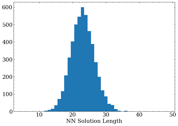 The caveat here is that it rarely, if ever, finds the shortest possible solution, which according to the DFS method should have an average length of around 12-13.
After several more hours of training, the network has reached its best performance (validated by letting it train overnight with no increase in performance), averaging around 18 moves per solution.
The caveat here is that it rarely, if ever, finds the shortest possible solution, which according to the DFS method should have an average length of around 12-13.
After several more hours of training, the network has reached its best performance (validated by letting it train overnight with no increase in performance), averaging around 18 moves per solution.
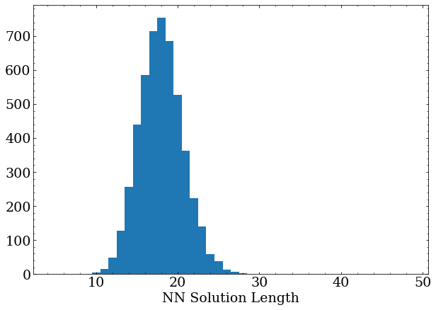 This is pretty impressive but still not entirely optimal compared to the actual-best solutions found by the DFS method.
That said, consider that this reinforcement learning method can be trained and solve several hundred thousand games with performance that I would consider comparable to a casual human player in the same time it takes the DFS approach to validate that there is no 15 move solution for a puzzle with a best solution length of 16.
This is pretty impressive but still not entirely optimal compared to the actual-best solutions found by the DFS method.
That said, consider that this reinforcement learning method can be trained and solve several hundred thousand games with performance that I would consider comparable to a casual human player in the same time it takes the DFS approach to validate that there is no 15 move solution for a puzzle with a best solution length of 16.
To improve this, a better network topology is an option, as is an improved reward calculation, or exploration strategy. So many options, and so little time!
>> Home