Previous solutions
Previously I wrote a depth first search (DFS) solver for the dust matching game pictured below, and have since done some thinking on how it might be solved more efficiently.
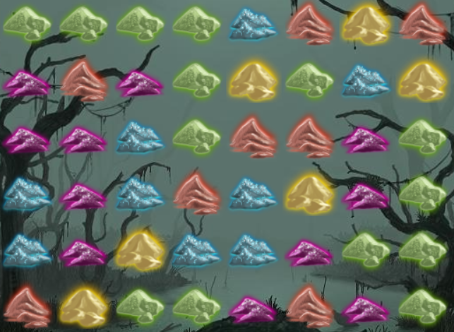 As a reminder, the rules of the game were that any similar color pile touching a pile of dust that is clicked are removed from the board, then the piles fall down and towards the center.
The DFS solver relied on a brute force method which would (eventually) find the ideal order in which to click dust clusters such that the board is cleared in a minimal number of moves.
The issue with this is that there are often more than 15 steps in the solution for a randomly generated board, and it can take an intractably long time for the solver to find the best solution, even with the help of several heuristics and shortcuts.
As a reminder, the rules of the game were that any similar color pile touching a pile of dust that is clicked are removed from the board, then the piles fall down and towards the center.
The DFS solver relied on a brute force method which would (eventually) find the ideal order in which to click dust clusters such that the board is cleared in a minimal number of moves.
The issue with this is that there are often more than 15 steps in the solution for a randomly generated board, and it can take an intractably long time for the solver to find the best solution, even with the help of several heuristics and shortcuts.
So the question becomes: how does one design the best heuristic, which is able to choose the correct cluster of colors to arrive at the shortest solution simply by looking at the current state of the board? In such a scenario, one would not require an exhaustive brute force search, but rather just show the board state to the heuristic and make the move it suggests. This is an ideal problem for neural networks, which are capable of modeling very complex classification problems. The primary difficulties with applying neural networks to this (or any) problem are:
- Choosing an appropriate network topology capable of learning the classification
- Presenting the network with sufficient training data to generalize to any arbitrary data
Network topology
Choosing a network topology is a very hard problem, and it is still very much the case in the field of machine learning that the correct topology is simply the one that performs the best. This leads to a lot of intuition, or even random assortment, being tested in a tiral-and-error way to find some reasonably well performing topology. My approach will be no better. What one can do prior to considering the topology of the network is decide on the input and output layers, which can inform your decision as to how to glue them together with a topology.
Input
The game is a 8 by 6 grid of numbers, so it should come as no surprise that the input will take the general form of an 8 by 6 tensor. Neural networks tend to perform best when each neuron (input) is related to some yes-or-no question. It is therefore beneficial to add a third axis to the input number that corresponds to the symbol present at the position specified by the first axis. It is an often overlooked mathematical fact that neural networks also perform better (especially in training) when the overall magnitude of the input remains mostly constant for different inputs. There are five colors (symbols) in this game, and also empty spaces, with board states near a solution consisting mostly of empty spaces. It is therefore a good idea for the third axis of the input to be length 6 where the 0th index will correspond to a blank space, and each color will be mapped to positions 1-5. Finally, the input should be one-hot representing the value at each grid location.
Altogether, this means the input tensor representing the state of the board will be shape where the first two dimensions are coordinates on the board, and the last dimension contains value for the index that corresponds to the symbol at the location. A 3D tensor is hard to represent visually, but suffice to say there are input values.
Output
Compared to the input, where there are 6 possibilities for each grid coordinate, the output is much simpler, and only needs to specify which location to click. Because there is often not a unique position for each possible move (anywhere on the same cluster is equally valid), and this is useful information for the network to understand, it is beneficial to highlight the whole cluster that is the correct one to click in the output. In practice, there will always be a best guess, or particular location within the correct cluster, reported by the network.
To encode this output, a single value should be specified at each grid location: 1 for the correct cluster and 0 for all other locations. This results in an tensor, or 48 values.
The middle bits
Certain classes of problems now have specialized network topologies that are known to perform well for the classifications the require. For instance, networks involving image processing are known to benefit from Convolutional Neural Networks (CNN), while networks involving time series data benefit from Long Short-Term Memory networks. One might think that this game distills down to some kind of generalized image, being a grid of values, and be tempted to use a CNN here. However, consider that CNNs leverage translational symmetry in images, meaning “information at the top” should be processed in roughly the same way as “information at the bottom” (or elsewhere). Such is not the case for this game, as the mechanic that pulls piles down and towards the center makes moves near the bottom have more side effects than moves near the top The game is also not really a time series (or any other kind of series), since only the current state matters in choosing the next move.
Without a good reason to use some tailored network topology, the general solution is to use a Dense network, which considers all possible connections between layers. These networks require a lot of training to determine which associations between neurons are useful, and what they should be, but they are excellent at “asking simple questions” about the data provided. The output of each neuron in a dense layer will be some weighted combination of the input to that layer, so it will qualitatively know things like:
- Are certain cells certain symbols
- Are there as many of these symbols as those symbols
- How many symbols left
- Etc.
This kind of information is not enough to base a guess for the next move on, but fortunately these layers can be stacked to ask more complicated questions about the initial data. While it is difficult to map out exactly what a network is doing, and I have no way of knowing a priori what a network will do, qualitatively neurons a second dense layer could answer more complicated questions about the simple inferences of the first layer.
Continuing this stacking for several iterations is the basis of Deep Neural Networks, and allows the last layer to ask very complicated questions. For CNN image processing, this can be as difficult as, “is a dog pictured in this image,” while for LSTM language processing one might ask, “what is the French equivalent of this English phrase.” Here the last layer of the dense stack is going to ask something along the lines of, “what information is needed to decide where to click next,” while the output layer will make the final decision based on that information.
After some limited fiddling, I decided (rather arbitrarily) that 10 dense layers with 1500 neurons each was both deep enough and contained a sufficient number of question-asking neurons to digest the information from the input and produce useful output.
The Keras model
Remaining decisions to make involve activation functions, loss calculation, and optimizer choice. For the stacked dense hidden layers, I choose to use the rectified linear unit (ReLU) activation function, as its linear region behaves nicely in deep networks, and is simple to calculate. Something like or other saturating functions were options here, but as these saturate to their constant values, the back-propagation of error tends to stall, resulting in a poorly optimized network. For the output layer, Sigmoid activation is attractive, because it produces output in the range , which can roughly be interpreted as a probability that the given neuron is the correct answer. Activation like Softmax are less suitable here, because they imply that the likelihood of one output being the answer influences the likelihood of other outputs, and this cross talk is less useful when calculating several nominally independent probabilities.
The loss here will be binary cross entropy, which is appropriate for a multiple label problem like this, where each grid location is labeled “click” (1) or “no-click” (0). The adaptive moment estimation (Adam) optimizer will be used, since it is robust to neurons that should be adjusted at different rates due to sparsity in the data, which can be thought of as allowing certain edge case solutions only used rarely compared to some general rule.
To create the model:
import tensorflow as tf
from tensorflow.keras import Input
from tensorflow.keras.layers import Dense
from tensorflow.keras.models import Model, load_model

width = 8
height = 6
nsym = 5

board_state = Input(shape=(width,height,nsym+1), name='board_state')
last = Flatten(name='flatten')(board_state)
for i in range(10):
    last = Dense(1500, name='hidden%i'%i, activation='relu')(last)
dense = Dense(width*height, name='dense', activation='sigmoid')(last)
board_guess = tf.reshape(dense,(-1,width,height),name='board_guess')
model = Model(inputs=[board_state], outputs=[board_guess])
model.compile(loss='binary_crossentropy',optimizer='adam')

model.summary()
Results from the summary printout:
Layer (type)                 Output Shape              Param #
=================================================================
board_state (InputLayer)     [(None, 8, 6, 6)]         0
_________________________________________________________________
flatten (Flatten)            (None, 288)               0
_________________________________________________________________
hidden0 (Dense)              (None, 1500)              433500
_________________________________________________________________
hidden1 (Dense)              (None, 1500)              2251500
_________________________________________________________________
hidden2 (Dense)              (None, 1500)              2251500
_________________________________________________________________
hidden3 (Dense)              (None, 1500)              2251500
_________________________________________________________________
hidden4 (Dense)              (None, 1500)              2251500
_________________________________________________________________
hidden5 (Dense)              (None, 1500)              2251500
_________________________________________________________________
hidden6 (Dense)              (None, 1500)              2251500
_________________________________________________________________
hidden7 (Dense)              (None, 1500)              2251500
_________________________________________________________________
hidden8 (Dense)              (None, 1500)              2251500
_________________________________________________________________
hidden9 (Dense)              (None, 1500)              2251500
_________________________________________________________________
dense (Dense)                (None, 48)                72048
_________________________________________________________________
tf_op_layer_board_guess_1 (T [(None, 8, 6)]            0
=================================================================
Total params: 20,769,048
Trainable params: 20,769,048
Non-trainable params: 0
Note that there are just under 21 million trainable weights in this model. This is on the large side for what is on the surface a relatively simple problem, but keep in mind that it nowhere near enough values to somehow represent a solution to any possible board configuration. This means that in order to perform well, the model will have to find general rules about which cell to click, which it will deduce during training.
Training dataset
Here’s the tricky part: one can’t just tell a neural network to learn to play a game, but rather one must show it how to play the game, and hope it can generalize from examples. This means that one must already have a selection of game states paired with the correct cluster to click to train this neural network. This raises the question: if you can generate solutions to create this training data, why bother creating this network? The bottom line here is that one can spend as much time and computing power as necessary to generate a library of board states and solutions, train the neural network on it, and then use the neural network to quickly find the solution to any other board. Since the depth first search brute force solver of the previous post can take hours to search all possible solutions, training the neural network, which could solve a board in several milliseconds, is a huge practical advantage.
So the goal here is to generate a library of boards and correct guesses. To do this, I will generate random boards, and solve them with some brute force depth first search solver. Each stage of the solution will be an separate input and output for the network to be trained on. In this case, since I’m working with Keras in Python, I’ve implemented the game logic from the previous post’s C++ Board class as a Python class:
class Board:
    def __init__(self,board=None):
        if board is None:
            self.board = np.random.randint(1,nsym+1,size=(width,height),dtype=np.uint8)
        else:
            self.board = np.copy(board)
    def copy(self):
        return Board(self.board)
    def _clear(self,x,y,val):
        if (x<0) or (x>width-1) or (y<0) or (y>height-1):
            return
        if self.board[x,y] == val:
            self.board[x,y] = 0
            self._clear(x-1,y,val)
            self._clear(x+1,y,val)
            self._clear(x,y-1,val)
            self._clear(x,y+1,val)
    def _contract(self):
        new = np.zeros((width,height),dtype=np.uint8)
        for x in range(width):
            col = self.board[x,:]
            col = col[col != 0]
            new[x,:len(col)] = col
        self.board = new
        new = np.zeros((width,height),dtype=np.uint8)
        for y in range(height):
            left = self.board[:width//2,y]
            left = left[left != 0]
            new[width//2-len(left):width//2,y] = left
            right = self.board[width//2:,y]
            right = right[right != 0]
            new[width//2:width//2+len(right),y] = right
        self.board = new
    def _cluster_flood(self,x,y,val,clusters,cluster):
        clusters[x,y] = cluster
        if x > 0 and clusters[x-1,y] == 0 and val == self.board[x-1,y]:
            self._cluster_flood(x-1,y,val,clusters,cluster)
        if y > 0 and clusters[x,y-1] == 0 and val == self.board[x,y-1]:
            self._cluster_flood(x,y-1,val,clusters,cluster)
        if x < width-1 and clusters[x+1,y] == 0 and val == self.board[x+1,y]:
            self._cluster_flood(x+1,y,val,clusters,cluster)
        if y < height-1 and clusters[x,y+1] == 0 and val == self.board[x,y+1]:
            self._cluster_flood(x,y+1,val,clusters,cluster)
    def clusters(self):
        clusters = np.zeros(self.board.shape,dtype=np.uint8)
        next_cluster = 1
        for y in range(height):
            for x in range(width):
                if clusters[x,y] == 0 and self.board[x,y] != 0:
                    self._cluster_flood(x,y,self.board[x,y],clusters,next_cluster)
                    next_cluster = next_cluster + 1
        return clusters
    def get(self,x,y):
        return self.board[x,y]
    def move(self,x,y):
        val = self.board[x,y]
        if val != 0:
            self._clear(x,y,val)
            self._contract()
        return self
    def remaining(self):
        return width*height - np.count(self.board == 0)
    def done(self):
        return np.all(self.board[:,0] == 0)
    def __str__(self):
        return '\n'.join([str(self.board[:,y])[1:-1] for y in reversed(range(height))])
A primary difference here is that I’ve generalized the game to any size board. I’ve only used 6 by 8 boards in this post, but I was working with smaller boards to in earlier testing, since the DFS solver is much faster for those. More on this later
The C++ DFS solver was also re-implemented as a python version:
def dfs_solve(b,history=[],max_depth=(width*height),verbose=False,max_time=None,start_time=None):
    if start_time is None:
        start_time = time.time()
    best_solution = None
    clusters = b.clusters()
    unique, counts = np.unique(clusters[clusters>0], return_counts=True)
    if len(history) < 6:
        guesses = [np.argwhere(clusters == guess_cluster)[0] for guess_cluster in unique]
        sortval = []
        for i,(x,y) in enumerate(guesses):
            guess_b = b.copy().move(x,y)
            guess_clusters = guess_b.clusters()
            guess_unique, guess_counts = np.unique(guess_clusters[clusters>0], return_counts=True)
            sortval.append(-counts[i]-np.max(guess_counts))
        sort = np.argsort(sortval)
    else:
        sort = np.argsort(-counts)
    ordered_clusters = unique[sort]
    ordered_guesses = [np.argwhere(clusters == guess_cluster)[0] for guess_cluster in ordered_clusters]
    for i,(x,y) in enumerate(ordered_guesses):
        if max_time is not None and time.time()-start_time > max_time:
            if verbose:
                print('max time',time.time()-start_time)
            return best_solution
        guess_b = b.copy().move(x,y)
        guess_history = history + [(x,y)]
        if guess_b.done():
            if verbose:
                print('solution len:',len(guess_history),'in:',time.time()-start_time)
            return guess_history
        else:
            if len(np.unique(guess_b.board))+len(guess_history) < max_depth: #if possible to clear faster than best
                guess_solution = dfs_solve(guess_b,guess_history,max_depth,verbose,max_time,start_time)
                if guess_solution is not None and len(guess_solution) < max_depth:
                    best_solution = guess_solution
                    max_depth = len(best_solution)
    return best_solution
While it is a bit slower than the C++ version in the brute-force regime, it is not significantly worse at finding the early solutions via heuristics.
I’ve also included a max_time parameter, which will truncate the search after a certain absolute time.
While this won’t be guaranteed to find the best solution in the the time limit, the limit can be chosen such that a pretty-good solution is found, which results in more training data for the network faster.
Some important caveats of this approach are discussed later.
Generating data
The first step is to generate a random board and solve it with the DFS solver. Here I’ve used a maximum time of 15 seconds, which rarely finds the absolute best solution, but there is a gulf of several minutes to hours between the solutions found in this time frame and better solutions, and I am not willing to wait that long for training data.
b = Board()
solun = dfs_solve(b,max_time=15)
A board state tensor for the neural network nn_in can then be constructed, utilizing fancy iteration from Numpy:
nn_in = np.zeros((width,height,nsym+1))
it = np.nditer(b.board, flags=['multi_index'])
for x in it:
    nn_in[it.multi_index+(x,)] = 1
The corresponding output tensor nn_out can be constructed from the first move in the solution, again with some Numpy magic:
move = solun[0]
nn_out = np.zeros((width,height))
clusters = b.clusters()
moves = np.argwhere(clusters == clusters[move])
for m in moves:
    nn_out[tuple(m)] = 1
But really what’s wanted here is a function that generates a whole batch for the Keras/Tensorflow model:
def gen_batch(dummy=None):
    batch_in = []
    batch_out = []
    while len(batch_in) < 500:
        b = Board()
        solun = dfs_solve(b,max_time=15)
        solun_b = b.copy()
        for move in solun:
            nn_in = np.zeros((width,height,nsym+1))
            it = np.nditer(solun_b.board, flags=['multi_index'])
            for x in it:
                nn_in[it.multi_index+(x,)] = 1
            nn_out = np.zeros((width,height))
            clusters = solun_b.clusters()
            moves = np.argwhere(clusters == clusters[move])
            for m in moves:
                nn_out[tuple(m)] = 1
            batch_in.append(nn_in)
            batch_out.append(nn_out)
            solun_b = solun_b.move(*move)
    batch_in = np.asarray(batch_in)
    batch_out = np.asarray(batch_out)
    return batch_in,batch_out
Here, I’ve ensured there are at least 500 board states per batch, which usually takes several minutes to complete.
Training the neural network
Mathematically speaking this is the hardest part of machine learning, but fortunately Keras and Tensorflow have abstracted away all the difficulty.
To keep things from take ages, I’ll run several copies of gen_batch in parallel, and pass those batches to the training code for the model.
An infinite while loop is used to train on 100 parallel-generated batches forever, or at least until someone hits Ctrl+C.
import multiprocessing as mp

while True:
    with mp.Pool(6) as p:
        for batch_in,batch_out in p.imap_unordered(gen_batch,range(100)):
            model.fit([batch_in],[batch_out],batch_size=len(batch_in))
Evaluating performance
Once the model is trained, it is straightforward to generate a board state tensor, run the model, and pick the coordinate in the output with the maximum value as the move to make.
b = Board()
while not b.done():
    nn_in = np.zeros((width,height,nsym+1))
    it = np.nditer(b.board, flags=['multi_index'])
    for x in it:
        nn_in[it.multi_index+(x,)] = 1
    nn_out = model.predict([np.asarray([nn_in])])[0]
    move = np.unravel_index(np.argmax(nn_out),nn_out.shape)
    b.move(*move)
With some additional printout code to show the symbol at each location on the grid with the neuron value times 100 (percent certainty) in parentheses, you can get an idea of what the neural network thinks the best guess and runner-up guesses are. Here’s an example of the neural network solving a board:
initial board:
  | 0     1     2     3     4     5     6     7
--+------------------------------------------------
5 | O( 0) B( 0) B( 0) G( 0) R( 0) B( 0) R( 0) Y( 0)
4 | G( 0) G( 0) Y( 0) Y( 0) Y( 0) R( 2) G( 2) R( 0)
3 | G( 0) O( 0) O( 0) Y( 1) O( 4) Y(17) O(25) G( 5)
2 | O( 0) Y( 0) G( 0) G( 3) O(17) R(57) R(63) O(22)
1 | G( 0) O( 0) Y( 0) R( 2) Y(15) Y(56) Y(69) Y(32)
0 | Y( 0) R( 0) R( 1) G( 2) O( 5) G(22) R(30) Y(12)
move 1: (6, 1)
  | 0     1     2     3     4     5     6     7
--+------------------------------------------------
5 | O( 0) B( 0) B( 0) G( 0)
4 | G( 0) G( 0) Y( 0) Y( 0) R( 0) B( 0) R( 0)
3 | G( 0) O( 0) O( 0) Y( 0) Y( 0) R( 0) G( 0) Y( 0)
2 | O( 0) Y( 0) G( 0) G( 3) O(13) Y( 4) O( 0) R( 0)
1 | G( 0) O( 1) Y( 9) R(52) O(79) R(64) R(17) G( 0)
0 | Y( 0) R( 2) R( 4) G(17) O(33) G(26) R(12) O( 2)
move 2: (4, 1)
  | 0     1     2     3     4     5     6     7
--+------------------------------------------------
5 | O( 0) B( 0) B( 0) G( 1)
4 | G( 0) G( 0) Y( 1) Y( 4) B(11) R(17)
3 | G( 0) O( 2) O( 6) Y(18) R(35) G(47) Y(40)
2 | O( 0) Y( 2) G( 3) G(21) Y(41) O(56) R(43)
1 | G( 0) O( 1) Y( 2) R( 6) R(21) R(32) R(30) G(13)
0 | Y( 0) R( 0) R( 2) G( 4) Y( 7) G(10) R(11) O( 6)
move 3: (5, 2)
  | 0     1     2     3     4     5     6     7
--+------------------------------------------------
5 | O( 0) B( 0) B( 0) G( 0)
4 | G( 0) G( 0) Y( 0) Y( 0) B( 2)
3 | G( 0) O( 0) O( 1) Y( 5) R(16) R(23) Y(14)
2 | O( 0) Y( 0) G( 2) G(19) Y(47) G(67) R(42)
1 | G( 0) O( 0) Y( 1) R( 7) R(27) R(45) R(33) G(10)
0 | Y( 0) R( 1) R( 2) G( 5) Y(12) G(19) R(16) O( 6)
move 4: (5, 2)
  | 0     1     2     3     4     5     6     7
-+------------------------------------------------
5 | O( 0) B( 0) B( 0) G( 0)
4 | G( 0) G( 0) Y( 0) Y( 0) B( 0)
3 | G( 0) O( 0) O( 0) Y( 0) R( 4) Y( 8)
2 | O( 0) Y( 0) G( 0) G( 5) Y(22) R(51) R(27)
1 | G( 0) O( 0) Y( 1) R( 9) R(38) R(68) R(59) G(14)
0 | Y( 0) R( 0) R( 2) G( 6) Y(14) G(31) R(29) O( 9)
move 5: (5, 1)
  | 0     1     2     3     4     5     6     7
--+------------------------------------------------
5 |       O( 0) B( 0) B( 0)
4 | G( 0) G( 0) Y( 0) G( 0)
3 | G( 0) O( 0) O( 0) Y( 0) B( 0)
2 | O( 0) Y( 0) G( 0) Y( 1) R( 0)
1 | G( 0) O( 0) Y(23) G(76) Y(16) Y( 0) G( 0)
0 | Y( 0) R( 2) R(11) G(47) Y( 4) G( 0) O( 0)
move 6: (3, 1)
  | 0     1     2     3     4     5     6     7
--+------------------------------------------------
5 |             O( 0) B( 0)
4 |       G( 0) G( 0) Y( 0)
3 | G( 0) O( 0) O( 0) B( 0) B( 0)
2 | O( 0) Y( 0) G( 3) G( 9) R( 7)
1 | G( 1) O(15) Y(63) Y(80) Y(70) Y(35) G(11)
0 | Y( 3) R(13) R(32) Y(54) Y(36) G(12) O( 5)
move 7: (3, 1)
  | 0     1     2     3     4     5     6     7
--+------------------------------------------------
5 |
4 |             G( 0) O( 0)
3 | G( 0) O( 0) G( 0) B( 0)
2 | O( 0) Y( 0) O( 0) Y( 0)
1 | G( 0) O( 0) G( 5) B( 0) B( 0) G( 0)
0 | Y( 0) R(38) R(87) G(15) R( 0) G( 0) O( 0)
move 8: (2, 0)
  | 0     1     2     3     4     5     6     7
--+------------------------------------------------
5 |
4 |                   O( 1)
3 |       G( 6) G(32) B(26)
2 | O( 0) O(57) G(89) Y(86)
1 | G( 0) Y( 3) O(15) B( 9) B( 0) G( 0)
0 | Y( 0) O( 2) G( 5) G( 2) R( 0) G( 0) O( 0)
move 9: (2, 2)
  | 0     1     2     3     4     5     6     7
--+------------------------------------------------
5 |
4 |                   O( 0)
3 |                   B( 0)
2 |       O( 0) O( 0) Y( 3)
1 | G( 0) Y( 0) O(13) B(62) B(60) G(13)
0 | Y( 0) O( 2) G( 5) G(22) R(21) G( 5) O( 2)
move 10: (3, 1)
  | 0     1     2     3     4     5     6     7
--+------------------------------------------------
5 |
4 |
3 |                   O( 0)
2 |       O( 0) O( 0) B( 0)
1 | G( 0) Y( 0) O( 0) Y( 2) G(42)
0 | Y( 0) O( 0) G( 0) G( 3) R(49) G(37) O( 5)
move 11: (4, 0)
  | 0     1     2     3     4     5     6     7
--+------------------------------------------------
5 |
4 |
3 |                   O( 0)
2 |       O( 0) O( 0) B( 1)
1 | G( 0) Y( 0) O(11) Y(63)
0 | Y( 0) O( 2) G(18) G(72) G(43) G( 4) O( 0)
move 12: (3, 0)
  | 0     1     2     3     4     5     6     7
--+------------------------------------------------
5 |
4 |
3 |
2 |             O( 3) O( 7)
1 | G( 0) Y( 5) O(65) B(61)
0 | Y( 2) O( 7) O(20) Y(15) O( 1)
move 13: (2, 1)
  | 0     1     2     3     4     5     6     7
--+------------------------------------------------
5 |
4 |
3 |
2 |
1 |             G( 1) B( 0)
0 |       Y(35) Y(93) Y(20) O( 0)
move 14: (2, 0)
  | 0     1     2     3     4     5     6     7
--+------------------------------------------------
5 |
4 |
3 |
2 |
1 |
0 |             G(45) B(99) O( 0)
move 15: (3, 0)
  | 0     1     2     3     4     5     6     7
--+------------------------------------------------
5 |
4 |
3 |
2 |
1 |
0 |                   G(99) O( 1)
move 16: (3, 0)
  | 0     1     2     3     4     5     6     7
--+------------------------------------------------
5 |
4 |
3 |
2 |
1 |
0 |                         O(99)
move 17: (4, 0)
Note here that the network cleared this board in 17 moves, in virtually no time. The DFS solver algorithm this was trained on only finds an 18 move solution in the 15 seconds allowed.
It is important to realize that this improvement over the algorithm it was trained on is mostly a fluke. In general, the network should only learn to approximate arbitrarily well the types of solutions it was shown. However, it is possible that, after seeing many slightly-sub-optimal solutions (because the DFS solver was truncated at 15 seconds), the network has generalized certain move-saving rules from other boards that applied to this board. As a general rule, if the training data continues to contain any sub-optimal solutions, the network will continue to consider that to be the target for optimal performance. So even if it occasionally teases out some rules to solve faster, these will be eventually lost in favor of the types of solutions it is trained on.
A statistical sample
Instead of looking at a particular solutions and comparing them step-by-step to the results of the DFS solver, a good way to monitor the training progress of the neural network (NN) is to compare the length of the NN solution to the length of the DFS solver solution for many random boards.
This is especially important since there are typically many unique solutions of the same length for any particular board, and we don’t care that the DFS solver and the NN solver found the exact same one, just that the NN is performing at least as well as the DFS.
With that in mind, here is a histogram of the solutions for the NN solver and the DFS solver for 1000 random boards that the neural network had never seen before.
For this plot the NN had been trained for roughly 24 hours on six cores, so roughly 35000 random boards, with around half a million individual board states.
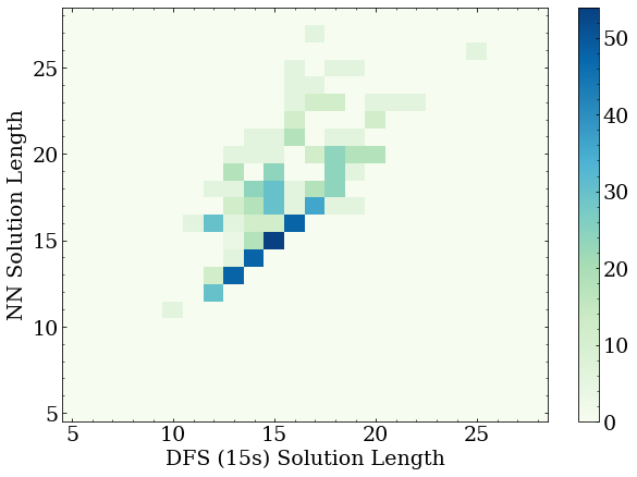 First, note that the majority of the boards are solved by the NN with the same number of moves as the DFS solver, as expected for a relatively well trained network.
These points fall on the diagonal line from bottom left to upper right.
Second, note that the NN solutions that were longer than the DFS solutions did terminate, and were within 7-10 moves of the DFS solution.
This is typical of the network making one or two less-than-optimal moves in the total move chain.
Third, note that there are several NN solutions that were better than the DFS solver, as exampled in the last section.
This is mostly a happy coincidence, as one cannot expect the NN to learn to solve any better than the dataset it is given.
First, note that the majority of the boards are solved by the NN with the same number of moves as the DFS solver, as expected for a relatively well trained network.
These points fall on the diagonal line from bottom left to upper right.
Second, note that the NN solutions that were longer than the DFS solutions did terminate, and were within 7-10 moves of the DFS solution.
This is typical of the network making one or two less-than-optimal moves in the total move chain.
Third, note that there are several NN solutions that were better than the DFS solver, as exampled in the last section.
This is mostly a happy coincidence, as one cannot expect the NN to learn to solve any better than the dataset it is given.
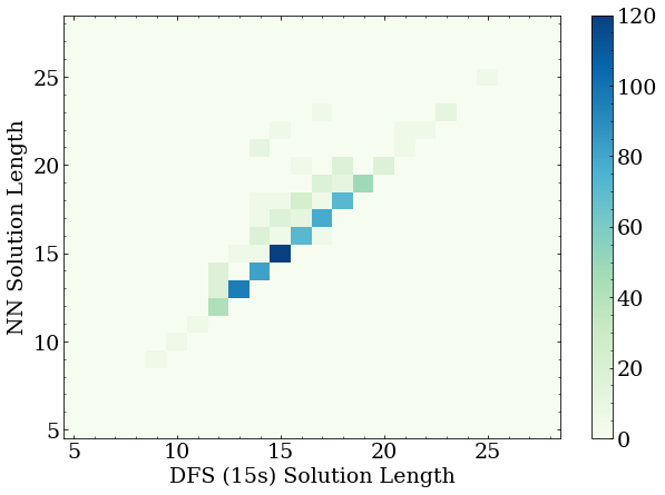
After another day of training, the NN solutions do indeed approach the DFS solutions much more reliably:
What next?
From here, more training with additional generated datasets would likely result in the NN reproducing the DFS solver solution lengths, with a few shorter flukes. This was observed with a similar topology on smaller boards. It would also be beneficial to find actual ideal solutions, and train the network on that, but this will require an enormous amount of computing power to generate the DFS solutions. A more exotic idea would be to now use the NN model as a heuristic, and try the “next-best” guess at every stage, to see if this leads to shorter solutions in any circumstances. If it did find shorter solutions with the next-best guesses, this could be used to generate a training set for the network. Repeating this process could allow the network to reinforce paths to shorter solutions, and out perform the time-limited DFS solver. This is a task for another time.
>> Home