Machine learning from scratch in Python with Numpy

Early in the Covid19 pandemic I decided to take a deep dive into the math and implementation of neural networks (NNs). Instead of treating NNs as a black box and using state-of-the-art packages like Tensorflow and Keras, which make NNs as accessible as LEGOs, I wanted to start from scratch and build the algorithms that Tensorflow (or any NN package) is based on. Historically this hands-on deep-dive learning style has worked quite well for me, and has resulted in some interesting projects like:

Lately I’ve found myself using Python more than any other language, and given its ubiquity in datascience, it’s an obvious choice for new projects. Some would complain that Python is slow, and to an extent these people are correct, but Python’s ability to integrate optimized native libraries sidesteps this issue, as long as you are willing to adopt the API/paradigm of these packages. NN math maps well onto matrix operations, and this is exactly the paradigm that the NumPy package has optimized and exposed to Python. What follows is a description of a neural network package based on NumPy, tensornetwork, that ended up being very similar in use to the Keras package mentioned earlier.

I also wanted to test a post that renders both highlighted code and mathematical expressions. Looks like it works nicely!

The Math

Neurons

The basic building block of the network is a neuron $N$ which accepts some input values, $x_i$, where $i$ is the index of the input, and has a single output value, $y$.

$$ N: x_i \rightarrow y $$

The function $N(x_i)$ is typically modeled as a nonlinear operation composed with a linear operation. The linear part typically takes inputs quantities and scales each by learned quantities, $w_i$ (weights), and sum the results with some learned constant, $b$ (bias). Note that this is essentially a dot product between vectors $\vec{x}$ and $\vec{w}$.

$$ z = b + \sum_i x_i w_i = b + \vec{w} \cdot \vec{x} $$

The nonlinear part, $\sigma(z)$, can be any nonlinear functions, where Sigmoid, $tanh$, or ReLU are common choices. The important part here is that the function is nonlinear, as a collection of linear operations can always be reduced to a single linear operation, and thus could not model nonlinear behavior. There is also a theorem demonstrating that connected nonlinear neurons can model any function. The functional form of a generic neuron can therefore be written as:

$$ y = N(\vec{x}) = \sigma(\vec{w} \cdot \vec{x} + b) $$

where $\vec{w}$ and $b$ are the learned quantities for the neuron.

Networks

Neural networks are collections of many neurons, $N_j(x_i)$, connected together, with some number of inputs $x_i$ and some number of outputs $y_j$ determined to suit a particular problem. It is common to think of large neural networks as a series of layers consisting of many neurons each. As best I can tell, this is done more for mathematical convenience than for any biological analog. While biological neural networks likely have feedback loops with outputs connected back to inputs that drive their output state, it is conceptually simpler to “unroll” or “flatten” this into a network with no loops (a feed forward network). In this paradigm, all the neurons in a layer share the same inputs, but weight these inputs differently:

$$ y_j = N_j(x_i) = \sigma_j\left(b_j + \sum_i w_{ji} x_i\right) $$

where the $j$ subscript indicates the $j$th neuron, such that $w_{ji}$ is the $i$th input weight for the $j$th neuron. Borrowing the previous notation the argument to the activation function $\sigma_j$ is:

$$ z_{j} = b_j + \sum_i w_{ji} x_i $$

If you take the $w_{ji}$ as the entries for a matrix $W$, this can be written as a matrix operation:

$$ \vec{z} = \vec{b} + W \cdot \vec{x} $$

where, if one assumes that the activation function is the same for all outputs in the layer and is applied to each element of the $\vec{z}$ vector, the layer expression can be written as:

$$ \vec{y} = \sigma(\vec{b} + W \cdot \vec{x}) $$

This expression is perfect for a math library like NumPy (and for hardware like GPUs) and can be written concisely:

output = activation(np.matmul(weights,inputs) + biases)

Learning

Backpropagation is the fundamental algorithm for updating the weights of each neuron incrementally such that the network approaches a configuration that results in the desired output for a given input. Reading the Wikipedia article will likely convince you that mathematical notation is confusing, but I’ll argue its the “bookkeeping” that is difficult, not the concepts. The conceptual idea is that a neural network with any weights produces some output for an input. If you know the desired output, you can compute an error between the true and desired output, and adjust the weights of the network to reduce this error. This is very similar to finding the minimum of some function (in fact, that’s all it is), with some caveats:

The number of parameters (weights and biases) can be very large for neural networks.
Each element in your dataset produces a different function to minimize, and you want the best minimum for all of them simultaneously.

Both points are addressed by making small corrections to the network for each element of a very large dataset of inputs and desired outputs.

Focusing on a particular neuron, with inputs $\vec{x}$, output $y$, and desired output $y_{true}$, you can define some error, $E$, based on the discrepancy in the output and desired output. A common choice is quadratic error $E = (y-y_{true})^2$, but cross entropy or more exotic options are possibilities. Don’t get too caught up on the particular choice for E, because that’s not what we want to know here. What we want is to know how to adjust the output of this neuron $y$ such that $E$ gets smaller.

The derivative $\frac{dE}{dy}$ is the mathematical expression for how much $E$ changes for a change in $y$, so if $\frac{dE}{dy}$ is positive, $E$ increases with larger $y$, meaning we want to decrease $y$ to achieve lower error. Since $y$ is a function of the inputs $\vec{x}$, weights $\vec{w}$ and bias $b$, we can consider adjusting any of these to reduce the error. So what we really want to know is, e.g. the derivative $\frac{dE}{dw_i}$, or the amount $E$ changes by for a change in the single weight $w_i$ (similarly $\frac{dE}{dx_i}$ for an input, or $\frac{dE}{db}$ for the bias).

Focusing on a particular weight, calculating the derivative $\frac{dE}{dw_i}$ requires only a little calculus (specifically, the chain rule):

$$ \frac{dE}{dw_i} = \frac{dz}{dw_i}\frac{dy}{dz}\frac{dE}{dy} $$

which is clear enough if you pretend you don’t know calculus, and treat infinitesimal quantities like $dy$ as a “small number” ($\frac{dy}{dy} = 1$). Given the formula for $z$ above, $\frac{dz}{dw_i} = x_i$ (similarly, $\frac{dz}{dx_i} = w_i$ for an input, or $\frac{dz}{db} = 1$ for the bias). Since $y = \sigma(z)$, $\frac{dy}{dz} = \sigma’(z)$ where $\sigma’$ is the derivative (slope) of the activation function. I will write this as $\sigma’_z$. Now we have expressions for the following derivatives:

$$ \frac{dE}{dw_i} = x_i\sigma’_z\frac{dE}{dy} $$ $$ \frac{dE}{db_i} = \sigma’_z\frac{dE}{dy} $$ $$ \frac{dE}{dx_i} = w_i\sigma’_z\frac{dE}{dy} $$

For output neurons $\frac{dE}{dy}$ can be directly computed from whatever expression is chosen for the error. In the simple case of quadratic error:

$$ \frac{dE}{dy} = 2(y-y_{true}) $$

For all other neurons, note that the $y$ outputs are $x_i$ inputs for other neurons. (Otherwise the outputs are unused, and the derivative of the error is zero). This means that $\frac{dE}{dy}$ for non-output neurons is the sum of the $\frac{dE}{dx_i}$ values, wherever the output $y$ is used as an input. This is where the “backpropagation” term comes from: first one computes the input derivatives $\frac{dE}{dx_i}$ for all neurons where $\frac{dE}{dy}$ is known, then repeats this procedure for the next layer up, and so on until all derivatives have been computed.

Once the derivative of the error is known with respect to each bias and weight in the network, a weight adjusting procedure can use these derivatives to adjust these parameters. The most straightforward is to adjust each weight (bias) by a small factor, $\epsilon$ of the derivative to arrive at a new weight $w_i’$ (new bias $b’$):

$$ w_i’ = w_i - \epsilon \frac{dE}{dw_i} $$ $$ b’ = b - \epsilon \frac{dE}{db} $$

More complicated adjustment algorithms such as RMSProp or ADAM use the same underlying math, but differ in the algorithm used to adjust the weights in the end.

As a final note, in most machine learning literature the error is called the “loss” and derivatives are referred to as “gradients”.

Where are the tensors?

Up to now I’ve only shown vectors and scalars as inputs and outputs to a neural network layer. Vectors are just tensors with a single index, and that’s all that’s necessary to describe inputs and outputs to single neurons or simple layers. When the input data has some dimensionality, i.e. grayscale images are 2D and RGB images are 3D, representing this dimensionality in the datastructure is convenient. Particularly when implementing layers like convolution layers, having the dimensionality manifest makes for more comprehensible code. Ultimately the calculations at the neuron level don’t care about the shape of your input data. For instance, the Dense layers implemented in tensornetwork allow arbitrary input tensor shapes, which are flattened, and the output can be any shape tensor that holds the number of outputs desired. Because all inputs are connected to every output, the shapes don’t change the calculation. Nevertheless, since Tensorflow works on tensors as layer inputs and outputs, I decided to implement something similar.

Code Organization

Taking the methodology in the previous sections, I’ve written Python code to implement the forward- and back-propagation math into layers commonly referred to in machine learning literature, including:

Dense fully connected layers
Conv layers with arbitrarily shaped kernels
Residual layers to model perturbations to the identity operator
LSTM and generic RNN recurrent layers featuring intra-layer connections
Pointwise layers that perform math on tensor elements

All tensornetwork submodules have their contents imported into the main module, which makes for more concise code, but makes it a bit harder to find the source.

The `network` module

High level structures describing a network as a collection of layers are defined here.

System class defines methods for interacting with an entire network
- Defining a network as a series of arbitrarily connected layers
- Saving and loading weights and biases
- Performing guess and learn operations
Structure class, which is the base class for all layer types
- Implements forward and backward operations for a layer.
- A __call__ on a Structure returns an Instance to store the neuron state
Instance class, which stores neuron state of a Structure within a System
- This abstraction allows may types of Structure to describe layers in a uniform way
- Several Instancess of a particular Structure can be independent
- Each instance stores its Structure to access the necessary calculations

The `neuron` module

Low level neuron calculations optimized for specific use cases. The base class NeuronNet implements the matrix calculation for a dense layer, which can be used as a building block for all other layer calculations. Certain types of layers have internal constraints which lend themselves to other optimizations for calculations. Simple examples include:

ConstantNet which simply injects constant values into a network not as a function of any inputs
ActivationNet which simply applies an activation function to input values without any neurons
Conv2DNet which uses optimized convolve and correlate operations instead of matmul given the kernel operation of 2D convolution is more efficiently represented this way than as a matrix multiplication.

The `activation` module

Contains several activation functions as subclasses of Activation which calculates:

The activation $a = \sigma(z)$ for a particular $\sigma$
The gradient $\frac{da}{dz}$ given the output activation $a$
- Coincidentally, most activation functions are monotonic with easy ways to express the gradient as a function of the output

Examples

The following example creates a network with 4 layers:

Input 32x32
Dense 15x15 with Tanh activation
Dense 15x15 with Tanh activation
Dense 26 with Sigmoid activation

import tensornetwork as tn

# Network parameters
input_shape = (32,32)
hidden_shapes = [(15,15)]*2
hidden_layers = len(hidden_shapes)
output_shape = ocr_data.out_shape

# Build Structures
in_layer = tn.Input(input_shape)()
last_layer = in_layer
print(in_layer)
for hidden_shape in hidden_shapes:
    last_layer = tn.Dense(hidden_shape,activation=tn.Tanh())(last_layer)
    print(last_layer)
out_layer = tn.Dense(output_shape,activation=tn.Sigmoid())(last_layer)
print(out_layer)

#Build System
s = tn.System(inputs=[in_layer],outputs=[out_layer])

The output shows the shapes of the tensors each layer expects:

Input :: [] -> [(32, 32)]
Dense :: [(32, 32)] -> [(15, 15)]
Dense :: [(15, 15)] -> [(15, 15)]
Dense :: [(15, 15)] -> [(26,)]

It is then possible to train this network on data:

for true_out,input in ocr_data.tagged_2d_data(length):
    guess_out,state = s.guess([input],return_state=True)
    s.learn(state,[true_out],method='adam',scale=0.0001,loss='ce')

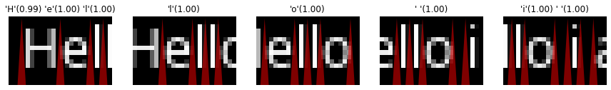
Optical character recognition benchmark

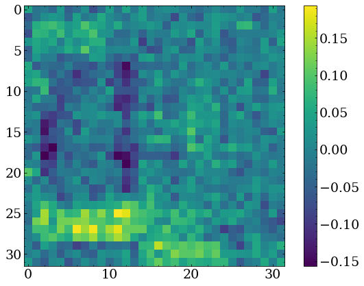Example weights for one neuron. The network built in the previous section was trained to identify upper case block letters represented as 32x32 grayscale images. After sufficient training, this achieves 100% accuracy, which is unsurprising given that there is limited variability possible in this benchmarking dataset. Looking at the weights of the neurons in the first dense layer, one can get an idea of the features the network is learning to recognize, for which an example is shown to the right.

Further examples

End-to-end OCR on blocky text similar to Oldschool Runescape Further examples can be seen with different types of neural network layers in the Jupyter notebooks in the tensornetwork repository. Particularly an end-to-end OCR example exists, which will (hopefully!) be a topic for a future post.

>> Home