Photorealistic rendering with global illumination from scratch

In a previous post I discussed the development and capabilities of the sdfray package, which represents scene geometries as signed distance functions (SDFs), and supports several rendering approaches. In this post, I’ll be discussing the rendering approach I previously called true optics, which tries to realistically simulate most commonly observed properties of light, to achieve a maximally realistic image. This falls under the umbrella of global illumination as it can accurately reproduce caustics and the effects of intra-illumination, which I would say is a bold enough claim to warrant some evidence.

I note here that I say most commonly observed properties of light because no wave effects (diffraction, thin film etc) are included — light is treated as distinct “photon” particles which travel like billiard balls through the scene. This is not uncommon for accurate optical simulations, as many physics-accurate simulations do the same for visible light, using phenomenological approximations for effects like thin film optics or diffraction when they are important, instead of directly keeping track of the phase of the light wave. Another departure from reality, that is tied to the nature of computer graphics, is that distinct red, green, and blue components of light are simulated. In principle you could think of these as averages over the wavelength distribution that activates red, green, and blue receptors in your eye. Perhaps it’s more accurate to think of these as the three distinct wavelength distribution produced by the pixels in your monitor. At any rate, this paradigm is insufficient for simulating effects of dispersion, like rainbows, or diffraction. Both effects would reveal the fixed nature of wavelength distributions. Also, general relativistic effects are not included, so no photo-realistic rendering of black holes, here (sorry).

Perhaps a future, truer optics will implement some of these effects, but having to deal with wavelengths makes aspects of the simulation much more difficult, as backtracking needs to have a hypothesized wavelength (or color) to be able to backtrack properly, which may not be possible if different wavelengths follow different paths. Let’s get into the approach to shed some light on this.

True optical simulation

The Monte-Carlo sampling approach of ray tracing a “photon” (I’ll drop the quotes from here on) in reverse is very effective at capturing the properties of light because optics is reversible (under most circumstances). So, given a photon arrived along a certain trajectory, that path can be traced backwards through the scene to figure out what color it should be. Nominally, this color is an average over all possible contributions, as all interesting things in physics are. It’s sufficient then to follow the ray back to a surface in the geometry, decide which optical process it undergoes at that surface (emission, transmission, specular reflection, diffuse reflection) according to some probability distribution, and continue the process along the incoming path, if necessary.

One simply needs to again average over the possible trajectories that can contribute to each pixel in the image. This average can be done at the same time by randomly sampling the geometry from random trajectories in the distribution for each pixel. Tens of thousands of samples may be needed for each pixel, leading to billions of paths that need tracing. This takes a long time compared to the time available to render a frame at 30fps, on any hardware, but frames can be rendered in “not too much time” using GLSL shaders and a relatively beefy GPU like an RTX 3090. I’ll get to some concrete examples, but minutes per frame is around the state of the art (at least with sdfray!), without going distributed or using more approximate lighting algorithms.

Random numbers in GLSL shaders

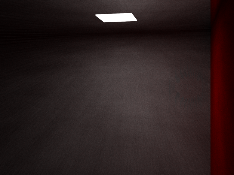
float rand(vec2 co) { // do not use this code, it's awfully bad
    return fract(sin(dot(co, vec2(12.9898, 78.233))) * 43758.5453);
}

Here co is a seed, typically the coordinates of the pixel being sampled, resulting in a pseudo random number derived from taking the fractional part of the sine of a rapidly changing function of the seed. The intuition here, as best I can tell, is that the fractional part is random because the number is so large and rapidly changing… needless to say that doesn’t hold up to scrutiny. Any way of creating a new seed from the result results in a very poor distribution of random numbers.

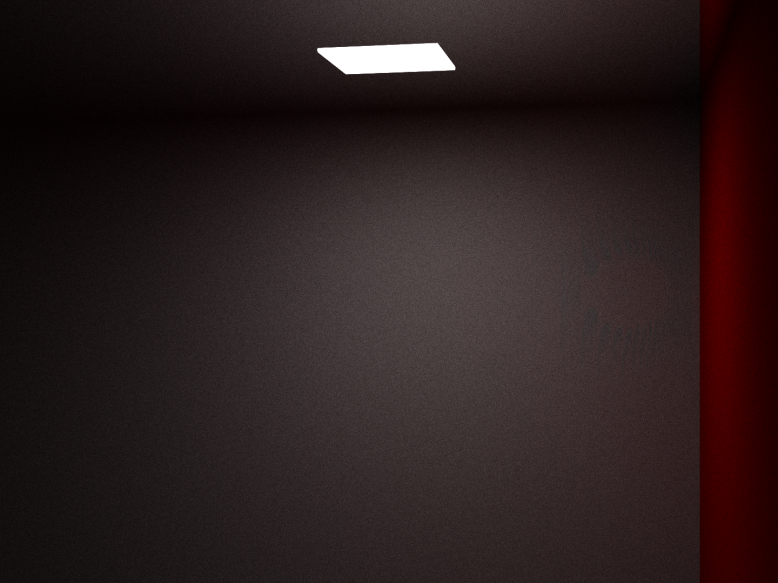
My GLSL implementation, along with seeding from the pixel coordinate (as is traditional), and a Box-Muller transform for normally distributed numbers, is given below.

uint pcg(uint v) {
    // https://www.pcg-random.org/
    uint state = v * uint(747796405) + uint(2891336453);
    uint word = ((state >> ((state >> uint(28)) + uint(4))) ^ state) * uint(277803737);
    return (word >> uint(22)) ^ word;
}
uint rnd_state;
void seed_rand(vec2 state) {
    rnd_state = pcg(pcg(pcg(floatBitsToUint(state.y))^floatBitsToUint(state.x))^floatBitsToUint(u_nonce));
}
float rand() {
    rnd_state = pcg(rnd_state);
    return float(rnd_state) / float(uint(0xffffffff));
}
float rand_normal() {
    return sqrt(-2.*log(rand()))*cos(2.*3.14159*rand());
}

u_nonce is a uniform that I change per-sample by sampling a much better RNG on the CPU, such that the GLSL RNG is seeded uniquely each time, ensuring uncorrelated sequences for each sample. Seeded this way, the PCG RNG will have long periods and excellent uniform distributions, independent for each sample, as evidenced by the image on the left above where the strange feature are now gone and a smooth (if grainy) background is present. Here, the grain is due to only using a limited number of samples per pixel, and is expected to improve with more samples.

Building up an image

To give some common baseline for comparison that’s a bit less esoteric than previous examples, I’ve implemented something like a Cornell room with: a checkered floor, a reflective sphere in the middle, and transparent glass-like cube and cylinder.

from sdfray.scene import Scene,Camera
from sdfray.geom import Union,Intersection,Subtraction
from sdfray.shapes import Sphere,Box,Cylinder,Plane
from sdfray.surface import UniformSurface,SurfaceProp,CheckerSurface
from sdfray.util import *

ctx = Context()
t = ctx['u_time']
ct = np.cos(t)
st = np.sin(t)
c = Camera(camera_orig=10*A([0,0,-1]),camera_yaw=0,width_px=960,height_px=720)

glossy = UniformSurface(SurfaceProp(diffuse=0.1,specular=0.8))
clear = UniformSurface(SurfaceProp(diffuse=0.05,specular=0.1,transmit=0.85,refractive_index=1.4))
red = UniformSurface(SurfaceProp(color=[1.,0.,0.]))
green = UniformSurface(SurfaceProp(color=[0.,1.,0.]))
blue = UniformSurface(SurfaceProp(color=[0.,0.,1.]))
bright = UniformSurface(SurfaceProp(emittance=[50,50,50]))

floor = Plane(anchor=[0,-2,0],normal=[0,1,0],surface=CheckerSurface(checker_size=0.25))
ceiling = Plane(anchor=[0,2,0],normal=[0,-1,0])
left = Plane(anchor=[-2.75,0,0],normal=[1,0,0],surface=blue)
right = Plane(anchor=[2.75,0,0],normal=[-1,0,0],surface=red)
back = Plane(anchor=[0,0,-2.75],normal=[0,0,1])
front = Plane(anchor=[0,0,2.75],normal=[0,0,-1])

light = Box(translate=[0,1.99,0],depth=1,height=0.02,width=1,surface=bright)

sdf = Sphere(translate=[0,-0.5,0],radius=0.8,surface=glossy)
sdf = Union(Box(translate=[-1.75*ct,0.5,-1.75*st],rotate=[0,3*t+2,2*t-1],depth=1.2,height=1.2,width=1.2,surface=clear),sdf)
sdf = Union(Cylinder(translate=[1.75*ct,0.5,1.75*st],rotate=[3*t+0.5,t+5,0],radius=0.6,height=1.2,surface=clear),sdf)

room_sdf = Union(floor,Union(ceiling,Union(left,Union(right,Union(front,Union(back,Union(light,sdf)))))))

s = Scene(room_sdf,[],cam=c)

If everything is working correctly, this should not only demonstrate both diffuse inter-reflection and caustics, but also showcase both in reflected and transmitted images.

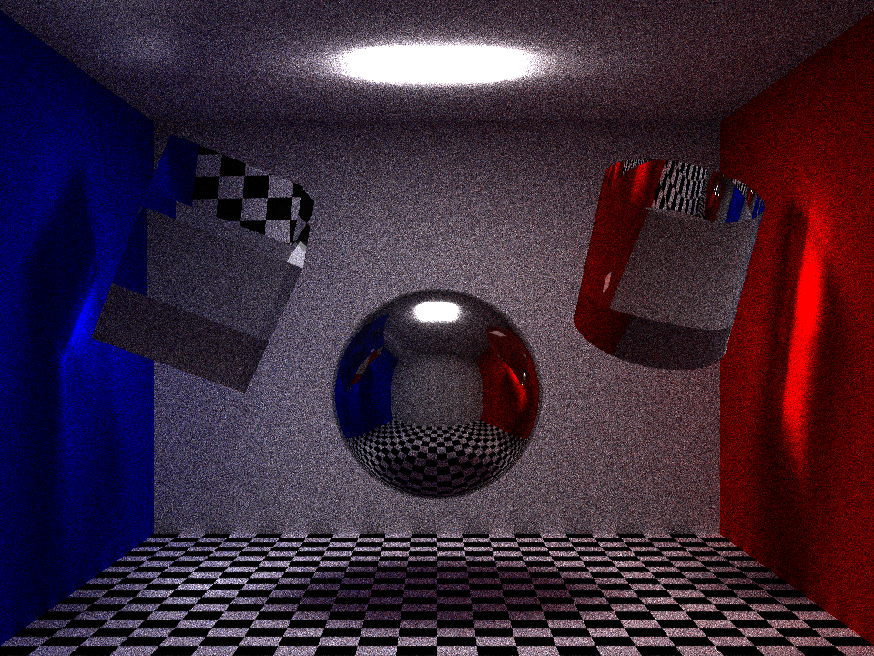
For illustrative purposes, averaging 10 samples, and using an angular uncertainty of 0.02 degrees for each pixel, results in this very sparse image:

s.clear_cache()
s.render(true_optics=True,ang_res=0.02,passes=10)

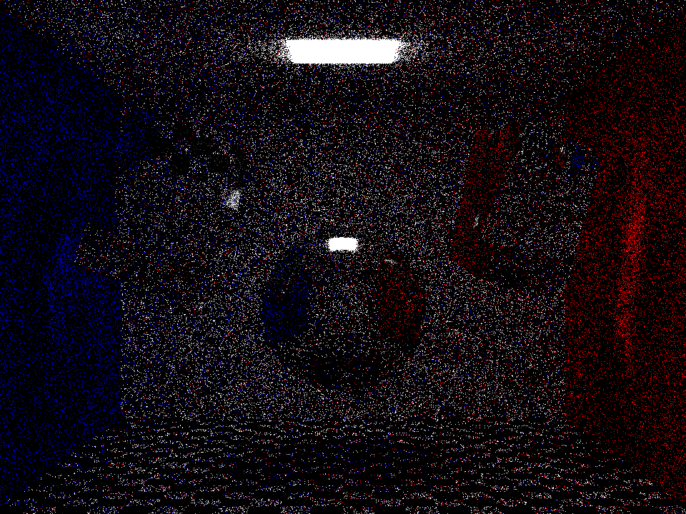
The light source is clearly defined, because every ray that terminates there samples the bright emitted light of that surface. Everything other point that is lit must have had a reflected ray land on the light source, after some number of bounces. The reflectivity (and color) of each intermediate surface modifies the observed color, such that the red wall begins to appear red. The white surfaces near the red wall also take on a red color, because some rays reflect off the wall before hitting the light. Many pixels are dark, because the series of reflections became too improbable to contribute significantly before hitting the light. Of note are slight evidence of caustics on the colored walls, and already clear specular reflection of the light source.

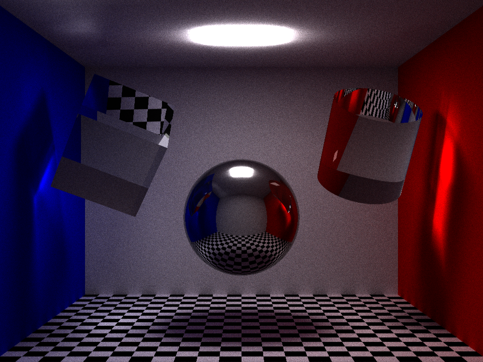
Moving on to 100 samples, the detail starts to become clearer:

s.clear_cache()
s.render(true_optics=True,ang_res=0.02,passes=100)

Edges of shapes are clear, and the transmitted and reflected images from the shapes can be made out. There are definite caustics, and even soft shadows are starting to appear. Notably, a blue to red gradient is forming on the white wall.

With 1000 samples, we can start to call this grainy instead of sparse.

s.clear_cache()
s.render(true_optics=True,ang_res=0.02,passes=1000)

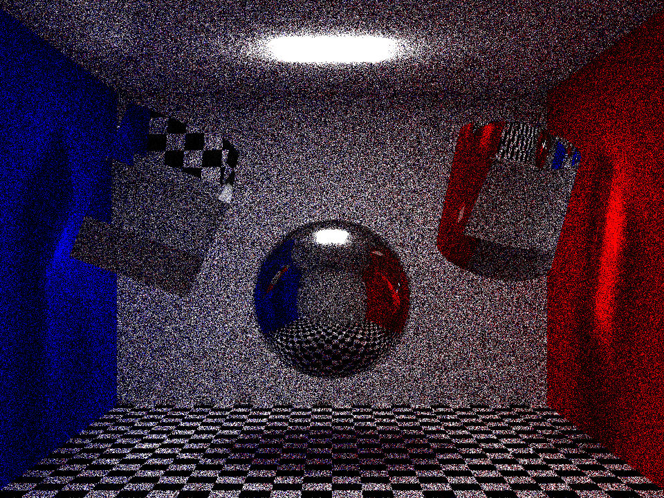
At 10k samples, this could be a photograph taken near Chernobyl subject to grain from intense radiation.

s.clear_cache()
s.render(true_optics=True,ang_res=0.02,passes=10000)

This many samples takes a few minutes for sdfray to render on a RTX 3090, which puts it somewhere around the maximum number of passes possible for frames of a video, depending on how patient you are, or how many GPUs you have.

Moving on to 100k samples, all the surfaces are smooth enough that I’m willing to call this photo-realistic. A bit of grain is still present, but we’ll chock it up to high ISO film.

s.clear_cache()
s.render(true_optics=True,ang_res=0.02,passes=100000)

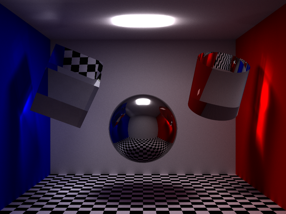
Fine detail is now visible in the caustics, which can also be seen reflected in the sphere. Very nice shadows are produced both by occlusion of the sphere and diversion of light by the transparent shapes. Further, the tiles can be seen to light the walls near them according to their lightness, resulting in a periodic illumination effect near the floor.

At a half hour or so, 100k samples per pixel comes close to exceeding my patience, but one could push it further for further reduced uncertainty in pixel colors. Video games with real-time raytracing typically don’t do this, and instead stick to a few hundred samples, and use AI or other techniques to infer the final image, which gets you there in reasonable time. Perhaps a project for another day!

From an image to a video

Using the same scene from above, and some slightly improved rendering code:

import io
import imageio
import base64 
from PIL import Image
from IPython.display import HTM

def encode_mp4(scene,times=np.linspace(0,2*np.pi,600),fps=60,framedir=None,**kwargs):
    try:
        os.mkdir(framedir)
    except:
        pass
    output = io.BytesIO()
    scene.clear_cache()
    with imageio.get_writer(output, format='mp4', mode='I', fps=fps) as writer:
        for i,time in enumerate(times):
            if framedir and os.path.exists(fname:=f'{framedir}/frame_{i:05d}.png'):
                v = Image.open(fname)
            else:
                v = scene.render(time=time,true_optics=True,**kwargs)
                if framedir is not None:
                    v.save(fname)
            writer.append_data(np.asarray(v))
    output.seek(0)
    return output.read()

def display_mp4(mp4,fname=None):
    if fname is None:
        b64 = base64.b64encode(mp4)
        src = f'data:video/mp4;base64,{b64.decode()}'
    else:
        with open(fname,'wb') as fout:
            fout.write(mp4)
        src = fname
    display(HTML(f'<video controls loop src="{src}"/>'))

A video of the scene in motion can be created, using 10k samples per frame here, which takes some considerable time to produce: around 2 days for a 10 second (600 frames at 60fps) video. Time taken aside, seeing the caustics move across the scene using code I wrote from scratch is quite satisfying. Perhaps time to look into some approximate techniques to boost the frame rate, and make the inclusion of more detailed optical properties a possibility.