I stumbled onto the concept of using signed distance functions (SDFs) to represent a three dimensional geometry almost by accident when looking up ways to generate 3D models (for 3D printers) programatically, as opposed to using traditional CAD software. Unlike more standard CAD processes for 3D printers, which tends to boil down to triangular meshes, SDFs are mathematical functions that can represent exact surface curvature. As I also have a background in physics-accurate optics I realized this property made SDFs ideal for high precision optical simulations, which is essentially the same thing as photo realistic rendering. It was immediately apparent with some quick googling that other people had previously explored the same ideas to great effect, but was interested enough that I got hooked, and decided to play around with writing my own rendering engine based on SDFs, and learn a bit along the way.
The sdfray renderer started as a few hundred lines of python code to find intersections of rays with an SDF.
It evolved into a pure-Python CPU rendering framework, using Numpy for the math, and finally into a Python framework for generating and running GLSL shader code for.
To help you understand what that means, I’ll dispense with the background knowledge first, then get into examples of the interesting bits.
Signed Distance Functions (SDFs)
Signed distance functions (you may see me use field and function interchangeably here) define the surface, or boundary, of an object by where some mathematical function goes through zero. They also possess the property that the value of the function is either the minimum distance to the surface or the negative of that if “inside” the object.
In general, such a function can be quite complicated, but for certain basic shapes, there are concise mathematical forms. A unit sphere at the origin is the simplest
where it is clear that the value is:
- at the origin - negative because inside, and one because the surface is one unit away,
- at the surface - is the usual definition for a unit sphere,
- the shortest distance to the surface, otherwise.
Inigo Quilez put together a nice article and many other resources with SDF implementations and techniques, which is worth checking out. These functions are interesting from a representational perspective for several reasons that deserve some discussion in the following sections.
Exact geometries
Most importantly to me, SDFs can represent a nonflat surface to arbitrary precision in a concise form, much unlike a triangular mesh that is popular in realtime computer graphics. This means that reflections and refraction won’t have to deal with flat surface approximations. It also means that for high detail one does not have to go to millions or billions of triangles on models, but rather define some function with sufficient detail. Because of this, signed distance functions have been used to study and display fractals, which have detail at all length scales.
Simple operations
Of algorithmic interest, there are simple methods for performing boolean operations on SDFs. The simplicity stems from SDFs being minimum distance fields. The SDF union of two SDF and is simply the lesser of the two SDF at any point
which tautologically means the nearest of the two surfaces is the closest surface.
There’s also an intersection operation resulting in the overlap of and .
which leverages the fact that SDFs are negative on the interior; the only remaining interior is where both interiors overlap, and the exterior is always the distance to the furthest surface.
Finally, the subtraction operation, to round out the constructive solid geometry, resulting in the boolean operation - , or with removed.
Here, the subtracting SDF is inverted, making its interior into exterior. The maximum, then, will always be the distance to on the exterior of , but wherever overlaps becomes exterior, since was negated.
With these operations, and a sufficient collection of primitive shapes, in principle any geometry can be constructed. Unfortunately, these CSG operations require evaluating both primitive (or composite!) SDFs, and on top of that have some issues with the interiors. It is important to recall that this is not the only way to construct SDFs, and indeed techniques like solids of revolution can perform better. As may people have explored this, I’ve stuck with CSG solids for demonstration purposes.
Fast ray intersection
Finally, and what inspired me to go further down the path of rendering, finding an intersection with a SDF geometry is a wholly different, and much faster, exercise than doing the same with triangular meshes. The latter is, of course, very simple, as one can directly calculate whether a ray intersects a triangle with well known formulas. The complexity comes with the sheer number of triangles one has to deal with, and the possibility that multiple triangles are intersected by the ray, but only one is visible.
For an SDF there is no general formula (though there are for specific cases) to calculate an intersection position. Instead, one can take advantage of the property that the value of the SDF is the minimum distance to a surface. There may not be a surface in the direction of the ray, but we know that the ray can be advanced by at least the value of the SDF without encountering any surface. Repeating this process will eventually result in either the value of the SDF approaching zero, meaning a surface has been encountered, or increasing forever, meaning there was no surface in the initial direction. This typically takes far fewer steps than there would be potential triangle intersections to calculate, making this potentially viable for real time raytracing or raycasting techniques. This, of course, relies on efficient evaluation of the SDF.
How much faster?
If the SDF is constructed from many operations on primitive shapes, single evaluations of the SDF could be many expensive floating point operations. The tipping point is probably somewhere around where the average number of steps necessary to find a surface, , times the complexity of the SDF evaluation, , approaches the number of triangles, , times the complexity of calculating a triangle intersection, . One could argue that is some primitive shape complexity, , times number of primitive shapes, , and could be something like number of primitive shapes, , times some average numer of triangles per shape, . With these made up variables, we favor SDF raytracing to triangle mesh raytracing when the following is true:
The complexity of intersecting a ray with one triangle is roughly the same order of magnitude as evaluating the SDF for one primitive shape. Both are pretty straightforward mathematical calculations. This means we an assume leaving
or that the average number of steps in finding an intersection should be less than the agerage number of triagles for simple shapes for SDFs to be competitive. When curved surfaces are involved, and high precision is needed there, this is often the case.
Raycasting and Raytracing
If you hold an empty picture frame in front of you, such tht some scene is contained within the frame, you have to look in particular directions from a particular location to see items withing the scene. In the same way, computer graphics are rendered by checking to see what color (and how bright) a particular part of the scene is, given a location and a direction. A location and a direction is a mathematical ray, and this checking of the scene color is the algorithm of raycasting, raytracing, or any number of techniques employed for creating computer generated images.
Typically this is an independent process for each pixel in an image; each pixel is cast as a ray to determin its color.
The Python and GLSL code fragments for this can be found in sdfray’s rendering core.
This proceeds according to the following rough outline:
1. Find an intersection
This is the stepping process where the SDF is evaluated at the point of a ray’s origin, and the value (minimum distance to a surface) is used to advance the ray until it encounters a surface.
For some batch of rays with properties for origins p and directions d and an sdf, some python code to do this follows:
WORLD_RES = 1e-4
WORLD_MAX = 1e4
def next_surface(p,d,sdf):
    alive = np.arange(len(p))
    intersected = np.zeros(len(p),dtype=bool)
    while len(alive) > 0:
        sd = sdf(p[alive])
        if np.any(m := (sd < WORLD_RES)): # hit something
            intersected[m] = True
            m = ~m
            alive = alive[m]
            sd = sd[m]
        if np.any(m := L(p[alive]) > WORLD_MAX): # infinity
            m = ~m
            alive = alive[m]
            sd = sd[m]
        p[alive,:] += (rays.d[alive].T*np.abs(sd)).T # advance batch
    return p,intersected
While the equivelant GLSL shader code would look something like:
float sdf(vec3 xyz) {
    // Since we can't pass a function by reference...
}

const float WORLD_RES = 1e-4;
const float WORLD_MAX = 1e4;
bool next_surface(inout vec3 p, inout vec3 d) {
    for (int i = 0; i < 2500; i++) {
        float v = sdf(p);
        if (v < WORLD_RES) {
            return true;
        } else if (v > WORLD_MAX) {
            return false;
        }
        p += v*d;
    }
    return false;
}
There are some additional considerations for a more robust method that can deal with low precision floating point math, where one might slightly over or undershoot, which can be found in the final codebase.
2. Determine the surface properties
My earliests tests were some few-hundred line long pure-python renderers with a hardcoded SDF which assumed all surfaces had the same diffuse reflectivity. The only frill was a bit of shading for the angle of the surface relative to a light source. Moving to something more complicated required a lot of infrastructure to keep track of surface properties. Not only are there multiple properties at each point, but different points may have to different sets of properties.
On the python side, it was fairly easy to have each primitive be an SDF object that had associated properties.
So when evaluating the SDF, one could simply query for the surface property at a point instead.
class SurfaceProp:
    '''Defines properties of a surface'''

    def __init__(self,color=A([1.0,1.0,1.0]),diffuse=0.8,specular=0.0,refractive_index=1.0,transmit=0.0,emittance=A([0.0,0.0,0.0])):
        '''Most quantities are multipliers for effects. [0,1] is realistic, but not required
           Refractive index is the usual way, where the speed of light in the medium is c/n
           Default surface is 80% diffuse reflective'''
        self.diffuse = diffuse
        self.specular = specular
        self.refractive_index = refractive_index
        self.transmit = transmit
        self.color = color
        self.emittance = emittance
In the GLSL code one is not fortunate enough to have objects and associated methods, but one does at least have structs.
The same properties can be represented as a struct, and another method sdf_prop constructed to re-evaluate the sdf for properties instead of distance.
struct Property {
    float diffuse, specular, transmit, refractive_index;
    vec3 color, emittance;
};

struct GeoInfo {
    float sdf;
    Property prop;
};

GeoInfo wrap(float sdf, Property prop) {
    return GeoInfo(sdf,prop);
}

GeoInfo wrap(GeoInfo info, Property prop) {
    return GeoInfo(info.sdf,prop);
}

Property sdf_prop(vec3 p) {
    return wrap(/* SDF HERE */,Property(1.,0.,0.,0.,vec3(1.,1.,1.),vec3(0.,0.,0.)));
}
Surface Normals
All the surface properties depend in some way on the orientation of the surface, because this influences how light illuminates a surface. It is therefore critical to exctract the surface normal vector - a vector that is unit length and perpendicular to the surface at a point. The distance properties of SDFs make this straightfoward: the gradient of the SDF , or , is equivelant to the surface normal at any point on the surface.
This is easy to compute in Python, using a central limit appoximation of the spatial derivatives,
D_ = 1e-4
DX = A([D_,0,0])
DY = A([0,D_,0])
DZ = A([0,0,D_])

def G(sdf,pts):
    '''Computes the gradient of the SDF scalar field'''
    return A([sdf(pts+DX)-sdf(pts-DX),
              sdf(pts+DY)-sdf(pts-DY),
              sdf(pts+DZ)-sdf(pts-DZ)]).T/(2*D_)
and isn’t any harder in GLSL.
const float D_ = 1e-4;
const vec3 DX = vec3(D_,0.0,0.0);
const vec3 DY = vec3(0.0,D_,0.0);
const vec3 DZ = vec3(0.0,0.0,D_);
vec3 gradient(vec3 p) {
    return vec3(sdf(p+DX)-sdf(p-DX),
                sdf(p+DY)-sdf(p-DY),
                sdf(p+DZ)-sdf(p-DZ))/(2.0*D_);
}
It is typical for the intersection code to pre-compute the gradient at the intersection point, to confirm it is in fact moving nominally torward the surface. Ultimately illumination from any source is proportional to the dot product of the direction to the source and the surface normal.
Diffuse reflectivity
Diffuse reflectivity models the reflected light that is reflected uniform in direction from a surface, giving surfaces their color. In principle, all light arriving at a surface is diffusely reflected in part back to the viewer, and must be taken into account. Therefore, handling diffuse reflectivity ammounts to accounting for all light arriving at a surface, if possible.
Specular reflectivty
Specular reflections are highly directional in nature, and the outgoing ray is in the same plane as and at the same angle from the normal vector. Accounting for specular reflection is therefore accounting for light arriving from a particular direction, which can be determined by the illumination of the surface in the direction of the reflection. This part is recursive, and requires running the full lighting stack for the reflected rays. Easy enough to do on a CPU, in GLSL this was accomplished with a finite stack and finite loop, each of sufficient size for non-pathological cases. Each step in the process usually has some inefficiency (nothing is 100% refective) so even in a very reflective environment, contributions from repeated reflections get smaller as the number of reflections increases.
Transmission
Transmission, particularly when refractive indices are different and refraction is significant, adds some complications. Foremost is that occlusion calculations relying on geometry intersection are no longer valid when surfaces may transmit. The fix to this also cannot be a straight line approximation through transparent objects due to refraction. Occlusion becomes a problem with no closed form solution, requiring iterative or exhausstive search methods to solve.
Of secondary consideration is that the renderer must either gracefully handle light being inside objects, or have a special case to determine an ultimate exit point, if one exists. I opted for the latter, just to get it working, but might revisit in the future. This then works like reflection, just from another direction and another point for the outgoing ray.
Going further
Not all reflections are exactly diffuse or exactly specular. What’s worse, reflectivity and transmission are linked and a fucntion of incidence angle for transmissive surfaces. We also know no real surfaces are perfectly smooth, which impacts everything discussed. These details could be improved for more realistic models, and indeed are included in simulations of optics within physics experiments.
3. Determine the lighting (color/brightness)
Eventually reflected and transmited rays will all terminate at some point where the lighting must be calculatd. I’ve explored two lighting schemes to go along with the SDF geometry and casting framework. The first is what I’ll call direct lighting where sources of light are defined, and the visibility of any point can be calculated by casting rays within the geometry. This method is very fast and is suitable for realtime demonstrations, but is limited in terms of the optical effects it can handle. The second I’ll call true optics where certain objects in the scene generate light, and the true behavior of light is simulated to light the image. While this can produce results indistinguisable from real life, it requires significantly more computation, and only appoximations (clever tricks) can get this running in real time.
Direct lighting
Since the discussion of surface properties indicates that all properties other than diffuse reflectivity are simply accounting for diffuse light from other surfaces, one needs only to account for how surfaces are lit in a diffuse sense to render an image. If a light has some color and is at some position , the surface at position with normal is illuminated by
where and are the direction and distance to the light, respectively. This holds as long as no other surface occludes the light from the perspective of the surface. A similar form for a distant light replacing with the value of direct illumination.
The inverse proportionality to the distance squared is a deep relationship to three dimensional geometry, and describes how the intensity of light decreases with distance. The dot product describes how the illumination of the surface with respect to the direction of the light is maximal when the normal and direction is aligned and behaves as for other angles. Finally, the illumination of the color of the surface is observed as a luminance
where denotes element-wise multiplication escribing the mixing of a color of light with a pigment, and is the emissivity property, that will be more important in the next section.
The approximations come in at two points: the occlusion calculation cannot handle complex light paths gracefully, and the description of light sources. Occlusion has partially been discussed, as it relates to finding refracted paths of light being difficult. A more subtle issue is that reflective surfaces can reflect light onto other surfaces, which isn’t accounted for at all, but falls under the umbrella of occlusion. The shortcomings related to light soruces are perhaps the most evident: point sources and directional/distant sources will produce knife edge shadows, which a keen eye will recognize as unrealistic.
Both of these approximations in light source and possible paths makes direct lighting deterministic and very fast. Surfaces where there’s a weighted mix of several effects simply produces the weighted result of those directly calculated effects. In many situations where caustics or illumination through a transparent/reflective surface isn’t present, this produces reasonable results, especially with techniques to smooth shadows. Indeed, this approach of backtracking rays through to diffuse surfaces to be illuminated is most similar to modern real-time rendering, where effects not reproduced by this approach are shoehorend in with approximations.
True optics
Fortunately, it’s possible to just get all the optics right with, in some sense, an easier approach, as long as you have copious amounts of processing power available. Understanding this is as simple as realizing this whole lighting exercise is “just” integrating the independent contributions of the entire scene. This integration problem can be solved with a traditional monte-carlo approach, tracing hypothetical photons back to where they came from to determine their intensity. This is similar to the direct lighting backtracking approach, but at a surface exactly on branch (transmit, diffuse, specular) is chosen, removing the recursive factor.
For diffuse reflection, instead of attempting to calculate the contribution of each light to the surface, a random reflection direction is generated and the tracing continues. The only way for the pixel corresponding to a ray to be lit is for this process to eventually land on a surface with emissivity . Before, this was just a color a surface had independent of illumination. Now, this is the only source of light.
Given the totally random nature of diffuse reflection, many traces will result in no emissive object being found. To produce an image, many hundreds or thousands of traces must be done to properly integrate the light sources, or some more intelligent integration technique must be used. Either way, while this produces all effects of light one might expect to see in real life, it is typically far too slow to employ without approximations in realtime applications.
sdfray rendering engine
Without further delay, the sdfray package implements the rendering fraemwork described in the previous sections, using signed distance function primitives to build a constructive solid geometry, and both direct and true lighting models.
I designed it to be easy to construct geometries in, and it is in a usable state for generating simple scenes.
sdfray is built on fairly standard Python packages, with the exception of ModernGL which I’ve found to be a refreshing and elegant way to run GLSL shaders, and highly recommend.
My ultimate goal in designing this was to get refraction working, and use it to render some caustics. To save you from clicking the link, caustics are light patterns produced by refracting or reflecting off a non-flat surface. This is an advanced feature of rendering, and not something typically taclked in game engines. Notably, the direct lighting style would have no chance of rendering a caustic, but it was crucial (in its speed) for testing and proving out the framework. With that in mind, I’ll step through some of the highlights along the development path.
Examples from sdfray
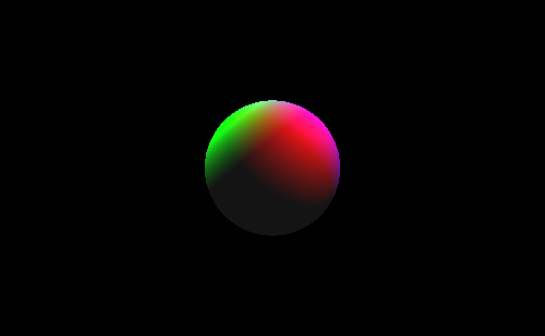
Probably the lowest bar is “can you render a sphere” for which the answer is assuredly yes, after some preliminaries.
from sdfray.light import DistantLight,PointLight,AmbientLight
from sdfray.scene import Scene,Camera
from sdfray.geom import Union,Intersection,Subtraction
from sdfray.shapes import Sphere,Box,Cylinder,Plane
from sdfray.surface import UniformSurface,SurfaceProp,CheckerSurface
from sdfray.util import *

import numpy as np
The general idea is that one defines the SDF for the geometry, and, if using the direct lighting model, some flavor of lights to illuminate the scene. The SDF is simple
sdf = Sphere()
where we’ve made heavy use of defaults, getting a unit sphere with a nominally diffuse surface.
This python object is callable to evaluate the SDF, and inherits from the SDF class to give it the ability to generate GLSL shader code, among other things.
I’ll generate several lights with different colors, one distant, and a bit of ambient lighting for contrast with the background.
lights = [
    PointLight([10,0,0],[2,2.5,-2]),
    PointLight([0,10,0],[-2,2.5,0]),
    DistantLight([0,0,1.5],[2,2.5,2]),
    AmbientLight([0.1,0.1,0.1])
]
From this, a Scene that can be rendered can be created.
Scene(sdf,lights).render()
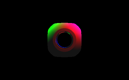
A slightly more complex demo of the CSG capability can be done.
cut_x = Cylinder(height=3,radius=0.5,rotate=[0,0,np.pi/2])
cut_y = Cylinder(height=3,radius=0.5)
cut_z = Cylinder(height=3,radius=0.5,rotate=[np.pi/2,0,0])
box_sphere = Intersection(Box(width=2,height=2,depth=2),Sphere(radius=1.2))
sdf = Subtraction(Subtraction(Subtraction(box_sphere,cut_x),cut_y),cut_z)

Scene(sdf,lights).render()
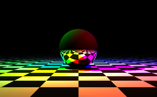
Showing off reflection capability is easier with something more complex still
glossy = SurfaceProp(diffuse=0.05,specular=0.85)
sdf = Sphere(radius=1.0,surface=UniformSurface(glossy))
demo_sdf = Union(sdf,Plane(surface=CheckerSurface()))
demo_lights = [
    PointLight([50,0,0],[2,2.5,-2]),
    PointLight([0,50,0],[-2,2.5,0]),
    PointLight([0,0,50],[2,2.5,2])
]
Scene(demo_sdf,demo_lights).render()
Adding in several shapes with different properties, including transmission.
mega_demo_lights = [
    PointLight([25,0,0],[2,2.5,-2]),
    PointLight([0,25,0],[-2,2.5,0]),
    PointLight([0,0,25],[2,2.5,2])
]

sdf = Sphere(translate=[0,-0.2,0],radius=0.7,surface=UniformSurface(SurfaceProp(diffuse=0.05,specular=0.05,transmit=0.9,refractive_index=1.4)))
sdf = Union(Box(translate=[-1.5,-0.2,0],depth=1.4,height=1.4,width=1.4,surface=UniformSurface(SurfaceProp(diffuse=0.9,specular=0.1))),sdf)
sdf = Union(Cylinder(translate=[1.5,-0.2,0],radius=0.7,height=1.4,surface=UniformSurface(SurfaceProp(diffuse=0.1,specular=0.9))),sdf)

mega_demo_sdf = Union(sdf,Plane(anchor=[0,-1,0],surface=CheckerSurface(checker_size=0.25)))
Scene(mega_demo_sdf,lights=mega_demo_lights,cam=Camera(width_px=1920)).render()
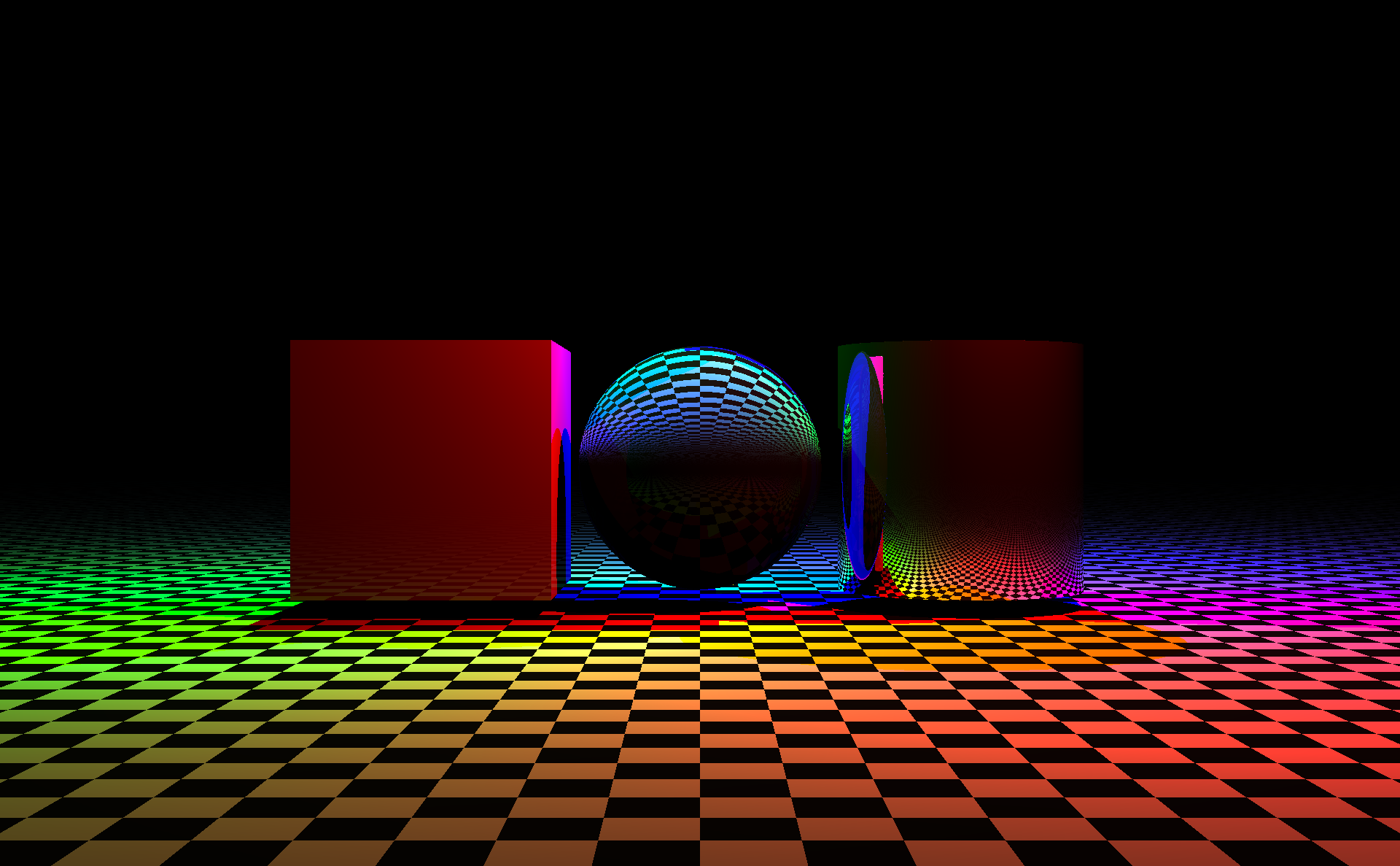
This is approximately the point at which the CPU renderer was too slow for rapid work, and I started moving towards GLSL.
Generating GLSL from the Python geometry is worth an entire other blog post, but suffice to say this opened up the possibility of adding motion in the form of per-frame parameters.
GLSL accomplishes this with uniforms which are values are passed to each thread of the shader rendering a scene.
I’ve adopted u_time as a value that increases every frame, and created a scheme for these parameters to be used in any part of the scene description.
This is a simple scene where the camera will orbit the origin.
ctx = Context()
t = ctx['u_time']
ct = np.cos(t)
st = np.sin(t)
c = Camera(camera_orig=10*A([st,0,-ct]),camera_yaw=-t,width_px=700)

s = Scene(Sphere(radius=1),lights,cam=c)
Rendering it requires some additional code, which I haven’t baked into sdfray yet, which handles the broiler plate task of encoding frames as an MP4 video.
import io
import imageio
import base64
from IPython.display import HTML

def encode_mp4(scene,times=np.linspace(0,2*np.pi,600),fps=60,framedir=None,**kwargs):
    try:
        os.mkdir(framedir)
    except:
        pass
    output = io.BytesIO()
    scene.clear_cache()
    with imageio.get_writer(output, format='mp4', mode='I', fps=fps) as writer:
        for i,time in enumerate(times):
            v = scene.render(time=time,**kwargs)
            if framedir is not None:
                v.save(f'{framedir}/frame_{i:05d}.png')
            writer.append_data(np.asarray(v))
    output.seek(0)
    return output.read()

def display_mp4(mp4,fname=None):
    if fname is None:
        b64 = base64.b64encode(mp4)
        src = f'data:video/mp4;base64,{b64.decode()}'
    else:
        with open(fname,'wb') as fout:
            fout.write(mp4)
        src = fname
    display(HTML(f'<video controls loop src="{src}"/>'))
Then we can render:
display_mp4(encode_mp4(s))
And at this point something can be designed that exceeds the capabilities of the direct lighting engine.
ctx = Context()
t = ctx['u_time']
ct = np.cos(t)
st = np.sin(t)
c = Camera(camera_orig=10*A([st,0,-ct]),camera_yaw=-t,width_px=704)

glossy = UniformSurface(SurfaceProp(diffuse=0.2,specular=0.8))
clear = UniformSurface(SurfaceProp(diffuse=0.05,specular=0.1,transmit=0.85,refractive_index=1.4))

sdf = Sphere(translate=[0,0,0],radius=0.9,surface=glossy)
sdf = Union(Box(translate=[-2,0,0],rotate=[0,3*t,2*t],depth=1.5,height=1.5,width=1.5,surface=clear),sdf)
sdf = Union(Cylinder(translate=[2,0,0],rotate=[3*t,t,0],radius=0.9,height=1.5,surface=clear),sdf)

clear_demo_sdf = Union(sdf,Plane(anchor=[0,-1,0],surface=CheckerSurface(checker_size=0.25)))

point_lights = [
    PointLight([50,0,0],[2,2.5,-2]),
    PointLight([0,50,0],[-2,2.5,0]),
    PointLight([0,0,50],[2,2.5,2])
]

s = Scene(clear_demo_sdf,point_lights,cam=c)

display_mp4(encode_mp4(s))
Looking carefully at the area under the rotating shapes, it can be seen that there’s more shadow that one would expect underneath a transparent shape. This is due to how the occlusion calculation is done in direct lighting engine. I’m only at the earliest stages of getting the true optics engine working well, but here is a teaser showing the promised caustics underneath the transparent shapes in the same scene.
display_mp4(encode_mp4(s,true_optics=True))
Several things to note about this render
- The grain is due to the random sampling of light paths in integration, and that I haven’t randomly sampled enough. There are 1000 samples per pixel here.
- The point lights have been converted to emissive spheres, which I grant are a bit silly, but give a good apples-to-apples comparison.
- The light patterns from refracted and reflected light below the transparent shapes meets my original goal.
There’s still a lot more I want to do with this, but it’s certainly at a satisfying place for now!
Realtime GLSL demos
This is a good time to highlight that the previous visualizations were MP4 videos, but modern browsers can render 3D content in realtime using WebGL.
Running a shader directly with WebGL is a bit of a pain, as I understand it, but frontends like glslCanvas make this painless.
What’s better: shader code generated by sdfray is almost drop in compatible with glslCanvas.
Here is one example showing off the accurate handling of refraction and reflection, realtime, using glslCanvas and WebGL.
Watch the sdfray repository for updates to the rendering engine, and check back for some deep dives into some of the capabilities listed here.