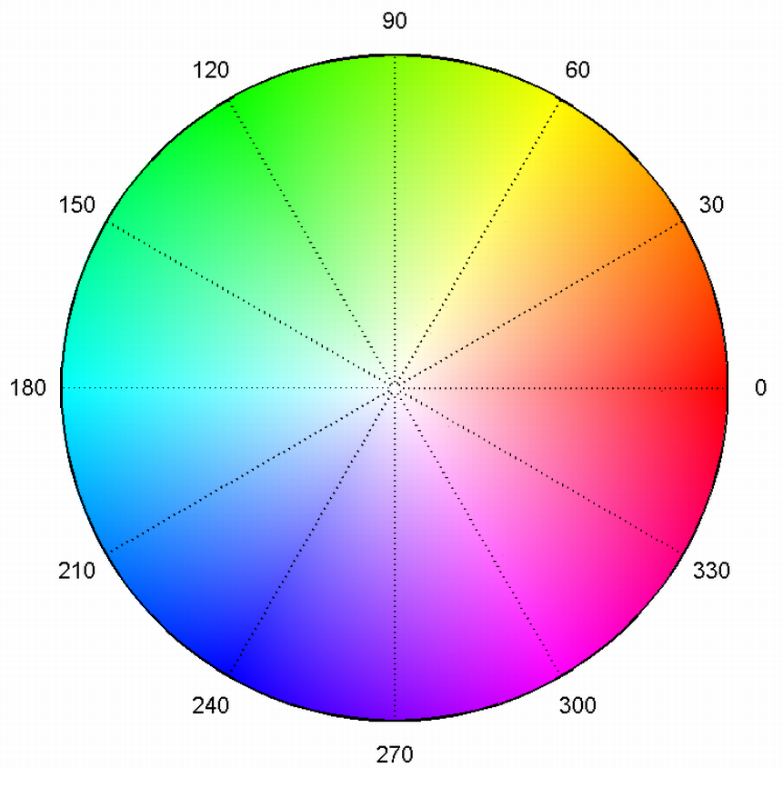
The HSV colorspace, matching angle to hue around the circle, and saturation to the radius.
In a previous post on simulating quantum mechanics, I visualized the complex numbers in the wavefunctions by plotting their real, imaginary, and magnitude (square root of probability) separately. As I mentioned briefly in that post, this is a bit lacking compared to the more intuitive way to think of complex numbers: as a magnitude and phase (angle). The magnitude was accounted for, but the real and imaginary parts can obfuscate the phase.
Like an angle, the phase is cyclic over radians or degrees. This can be represented by some cyclic color map, as easily as mapping the phase to the hue of a color in the HSV color space, which can make for a visually more intuitive representation of the phase.
Using this scheme, I’ve opted to shade below the magnitude with a hue determined by the phase, and re-rendered the results from the previous post. As a bonus, I have also extended the simulation into two dimensions, and added GPU acceleration, which I’ll discuss in the last half.
Wave functions in one dimension
The figures in this section are identical wave functions as those in the previous post, but visualized with the phase as hue. Having matplotlib shade under a regular plot as a function of position proved challenging, so I oped for adding the shading to a plot manually.
import numpy as np
import matplotlib.pyplot as plt
from matplotlib.colors import hsv_to_rgb

def polygon(x1,y1,x2,y2,c,ax=None):
    if ax is None:
        ax = plt.gca()
    polygon = plt.Polygon( [ (x1,y1), (x2,y2), (x2,0), (x1,0) ], color=c )
    ax.add_patch(polygon)

def complex_plot(x,y,ax=None,**kwargs):
    mag = np.abs(y)
    phase = np.angle(y)/(2*np.pi)
    mask = phase < 0.0
    phase[mask] = 1+phase[mask]
    hsv = np.asarray([phase,np.full_like(phase,0.5),np.ones_like(phase)]).T
    rgb = hsv_to_rgb(hsv[None,:,:])[0]
    cmap = plt.get_cmap('hsv')
    if ax is None:
        ax = plt.gca()
    ax.plot(x,mag,color='k')
    mask = mag > np.max(mag)*1e-2
    [polygon(x[n],mag[n],x[n+1],mag[n+1],rgb[n],ax=ax) for n in range(len(x)-1) if mask[n] and mask[n+1]]
    ax.set_xlabel('Position')
    ax.set_xlim(-2,2)
    ax.set_ylim(0,None)
Note that the axis is an optional argument, which proved critical when producing animated visualizations.
from matplotlib.animation import FuncAnimation

def animate(simulation_steps,save_as=None,init_func=None):
    fig, ax = plt.subplots()
    complex_plot(x,simulation_steps[0],ax=ax)
    ax.set_xlim(-2,2)
    ax.set_ylim(0,4)
    if init_func:
        init_func(ax)

    def animate(frame):
        ax.clear()
        complex_plot(x,simulation_steps[frame],ax=ax)
        ax.set_xlim(-2,2)
        ax.set_ylim(0,3)
        if init_func:
            init_func(ax)

    anim = FuncAnimation(fig, animate, frames=int(len(simulation_steps)), interval=50)
    plt.close()

    if save_as:
        anim.save(save_as, writer='imagemagick', fps=30)

    return anim
For the rest of the code and commentary, see the previous post. I’ll just be reproducing the plots here.
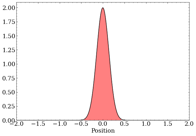
A wave packet with zero momentum is just a real-valued Gaussian distribution. These are complex numbers with the same phase but differing magnitude
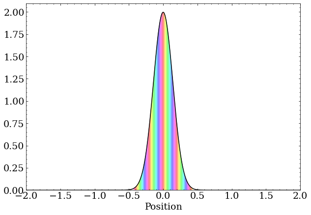
A wave packet with nonzero momentum still has a magnitude that is a Gaussian distribution, but the complex phase changes as a function of position at a rate proportional to the momentum.
A free, stationary particle
A free particle with momentum
A particle in a box
A particle encounters a barrier
A particle in a quadratic potential
Quantum harmonic oscillator eigenstates
Evolution of a guess to the three lowest energy states:
Time evolution of the second excited state:
Wave functions in two dimensions
I first started playing with phase as hue when trying to visualize a 2D wavefunction. The major difference, of course, now having four dimensions to visualize: two spatial dimensions, along with the magnitude and phase at every point. The generalization of the previous plot would be a two dimensional surface in 3D with the third dimension being the magnitude, and shaded with a hue to represent the phase. Without going to a 3D plot, I opted to stick with the HSV color space and make an image with two axes for space and the the hue for phase and value for magnitude. This way, large magnitudes are brighter, colored by the phase, which makes for some impressive visualizations.
Of course, simulating in 2D requires changes, including a way to deal with the a wavefunction on a 2D grid as opposed to a 1D grid. First of all, since integrating the Schrodinger equation in 2D will be much more computationally intense than in 1D, I’ll be using Cupy to accelerate most of the math with a GPU. This ultimately makes the 2D simulations take less time than the 1D simulations, though the smallness of the data in 1D means GPU acceleration would not help much.
import numpy as np
import cupy as cp
import matplotlib.pyplot as plt
This will be the definition of the 2D grid the wavefunction will be sampled on.
x = cp.linspace(-10,10,500)
y = cp.linspace(-10,10,500)
extent = cp.asnumpy(cp.asarray([cp.min(x), cp.max(x), cp.min(y), cp.max(y)]))
xv, yv = cp.meshgrid(x, y, indexing='ij')
deltax = x[1]-x[0]
deltay = y[1]-y[0]
deltaxy = deltax*deltay
And here is a way to normalize a wavefunction in 2D
def norm(phi):
    norm = cp.sum(cp.square(cp.abs(phi)))*deltaxy
    return phi/cp.sqrt(norm)
which is equivalent to satisfying the condition
and might be written by a physicist as
to generalize into any number of dimensions.
Wave packets
To build an analogous wave packet to the 1D case, one uses a Gaussian profile in both spatial dimensions, and the rate of change of phase in each direction encodes momentum in that direction.
def wave_packet(p_x = 0, p_y = 0, disp_x = 0, disp_y = 0, sqsig = 0.5):
    return norm( cp.exp(1j*xv*p_x) * cp.exp(1j*yv*p_y)
                *cp.exp(-cp.square(xv-disp_x)/sqsig,dtype=complex)
                *cp.exp(-cp.square(yv-disp_y)/sqsig,dtype=complex))
And to display these beauties, the magnitude is converted into a value (brightness) and phase into a hue. I choose a low saturation, here, as before, before because fully saturated hues diminished the ability to perceive the change in magnitude encoded in the value.
from matplotlib.colors import hsv_to_rgb

def to_image(z,z_min=0,z_max=None,abssq=False):
    hue = cp.ones(z.shape) if abssq else cp.angle(z)/(2*cp.pi)
    mask = hue < 0.0
    hue[mask] = 1.0+hue[mask]
    mag = cp.abs(z)
    if z_max is None:
        z_max = cp.max(mag)
    if z_min is None:
        z_min = cp.min(mag)
    val = (mag-z_min)/(z_max-z_min)
    hsv_im = cp.transpose(cp.asarray([hue,cp.full_like(hue,0.5),val]))
    return hsv_to_rgb(hsv_im.get())

def complex_plot(z,z_min=None,z_max=None,abssq=False,**kwargs):
    plt.xlim(-2,2)
    plt.ylim(-2,2)
    return plt.imshow(to_image(z,z_min,z_max,abssq),extent=extent,interpolation='bilinear',**kwargs)
With that, some simple cases can be plotted.
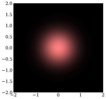
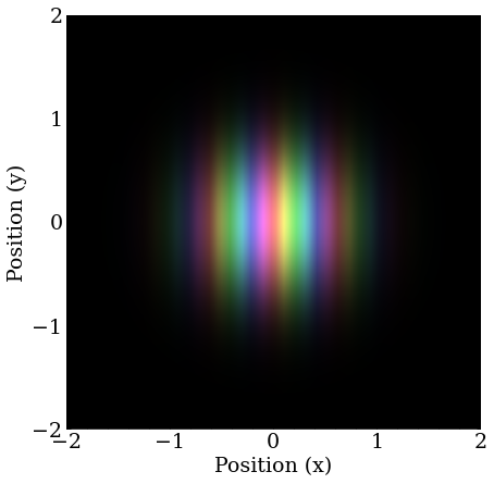
A wave packet with zero momentum is just a real-valued Gaussian distribution in two dimensions. These are complex numbers with the same phase but differing magnitude
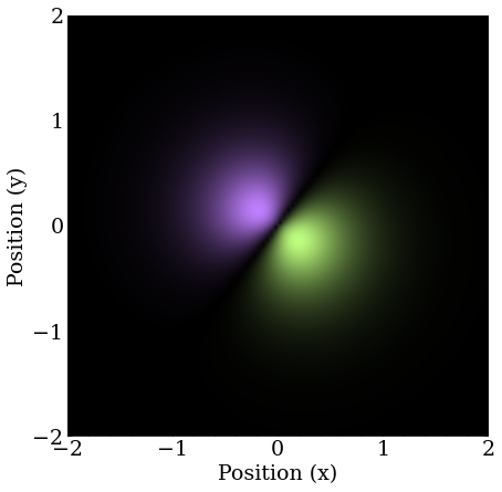
A wave packet with nonzero momentum still has a magnitude that is a 2D Gaussian distribution, but the complex phase changes as a function of position at a rate proportional to the momentum. Only momentum in the X direction is shown here
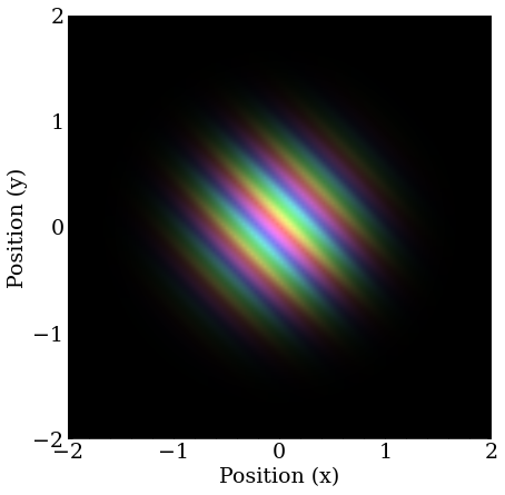
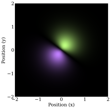
Similar to the previous, but with equal amounts of momentum in the X and Y directions.
For time evolution, the code is much the same, except now potentials are a function of the 2D grid, and momentum can be in the X or Y directions. The code for computing the time derivative can actually remain almost the same
def d_dt(phi,x=x,h=1,m=1,V=0):
    return (1j*h/2/m) * gradsq(phi) - (1j/h)*V*phi
where the gradsq or is notation generalizes the second derivative of space to higher dimensions.
More formally, is a vector of derivative operators, with as many dimensions as the situation requires, often call the gradient of a function.
And it is understood that it behaves similar to an operator when “multiplying.”
Applying to a vector field instead of a scalar field, often called the divergence is more like a dot product of and the vector. Because is a vector, , sometimes called the Laplace operator can be thought of as
where it is clear that in 1D this is the correct second derivative of position, and the intuition that this is proportional to the kinetic energy suggests the addition of a similar kinetic energy term in the y-direction is appropriate for the total kinetic energy.
With that, that the generalized multi-dimensional Schrodinger equation becomes the following.
The gradsq function implemented with the same trick in the y-direction as was previously used in the x-direction, where I’ve combined the central values from the two derivatives to reduce the number of matrix operations.
def gradsq(phi):
    gradphi = -4*phi
    gradphi[:-1,:] += phi[1:,:]
    gradphi[1:,:] += phi[:-1,:]
    gradphi[:,:-1] += phi[:,1:]
    gradphi[:,1:] += phi[:,:-1]
    return gradphi
The exact same time evolution methodology from the previous post can be used with this new time derivative, since the Numpy arrays handle the generalization to 2D wavefunctions (and higher) gracefully.
A free, stationary particle
Much like the 1D case, a stationary, localized particle spreads out in time. As the particle spreads into two dimensions, the reduction in magnitude everywhere to preserve the normalization is dramatic.
A free particle with momentum
A particle with momentum behaves as expected, and in 2D, curved wavefronts can be seen as the packet disperses.
A particle in a box
I almost did not include this, because its a mess, and not very intuitive to the uninitiated, but it’s a mesmerizing visual. Interference fringes can be seen in both directions, now, as the particle bounces off all four walls of the 2D box. Otherwise, this is quite similar to the outcome of the 1D case, getting interference patterns similar to eigenstates after the particle’s location is fully scrambled.
A particle encounters a barrier
The barrier, here, is at is between and is higher potential than the classical energy of the particle, just like the 1D case.
V_barrier = cp.where(cp.logical_and(xv>2.5,xv<2.75),9e-2,0)
The component that tunnels through can be seen, while the bulk reflects.
A particle in a 2D quadratic potential
A 1D quadratic potential in 2D would show dispersion in the unconstrained direction, but a 2D model lets particles bounce back and forth with the same reasoning as before.
V_harmonic = 2e-2*(cp.square(xv)+cp.square(yv))
This example starts from the origin with a momentum in the x-direction.
Here the particle is offset, to give it some angular momentum, driving home the 2D nature of this simulation. The “orbit” is not perfect, since I only eyeballed the radius and angle, but it makes it around a few times, unperturbed. Note, also, how the direction of the gradient in phase is changing with the momentum, as it should.
Coulomb potential eigenstates
The Coulomb potential of charged particles (and many other phenomenon) becomes interesting in two dimensions, and one can start to think of even generalizing to three dimensions to simulate a hydrogen-like atom. Before going there, one can utilize the complex time evolution technique to find eigenstates of this more interesting potential, which takes the form of an inverse square law.
The Coulomb potential is scaled here to a magnitude that makes sense for these visualizations.
V_coulomb = -1e-2/np.sqrt((cp.square(xv)+cp.square(yv)))
Being a bit more pragmatic than before, I’ve put together a function to find the next lowest state given some guess containing it, and a list of states to maintain orthogonality with.
def find_next_eigenstate(psi_guess, eigenstates=[], adaptive=1.0, tol=1e-10, steps=50000, dt=-1e-1j, V=V_coulomb,**kwargs):
    condition = orthogonal_to(eigenstates)
    psi_guess = condition(psi_guess)
    complex_plot(psi_guess)
    plt.show()
    plt.close()
    sim_states,eig = simulate(psi_guess,
                              dt = dt,
                              steps = steps,
                              adaptive = adaptive,
                              V = V,
                              condition = condition,
                              tol=tol,
                              **kwargs)
    complex_plot(eig)
    plt.show()
    plt.close()
    return sim_states,eig
This uses a more advanced version of the original simulate method, which includes a tol parameter for aborting the simulation if the difference of the two wavefunctions has a magnitude of at most tol at any point.
This improved simulate also allows for an adaptive step size which scales the step size dt by where is the same maximum magnitude of the difference between the last two time steps compared to tol, and is the tuning factor adaptive.
This lets the simulation take larger steps, proportional to the logarithm of the difference, when the difference is small, and the corresponding error of the integration will be small, converging faster to the ground state.
def simulate(phi_sim, method='rk4', V=0, steps=10000, dt=1e-1, adaptive=None, condition=None, normalize=True, plot_every=None, save_every=50, tol=None):
    simulation_steps = [phi_sim.get()]
    tol_cur = 1.0
    for i in range(steps):
        if adaptive is not None:
            dt_now = -adaptive*np.log10(tol_cur)*dt if tol_cur < 1.0 else dt
        else:
            dt_now = dt
        if method == 'euler':
            phi_next = euler(phi_sim,dt_now,V=V)
        elif method == 'rk4':
            phi_next = rk4(phi_sim,dt_now,V=V)
        else:
            raise Exception(f'Unknown method {method}')
        if condition:
            phi_next = condition(phi_next)
        if normalize:
            phi_next = norm(phi_next)
        if tol is not None:
            if (tol_cur:=np.max(np.abs(phi_sim-phi_next))) < tol:
                return simulation_steps,phi_next
        phi_sim = phi_next
        if save_every is not None and (i+1) % save_every == 0:
            simulation_steps.append(phi_sim.get())
        if plot_every is not None and (i+1) % plot_every == 0:
            print(i, dt*i)
            print(tol_cur)
            complex_plot(phi_sim)
            plt.grid()
            plt.show()
            plt.close()
    return simulation_steps if tol is None else (simulation_steps,None)
I’ll be using an initial guess with some momentum in both the x and y directions with a bit larger initial size, to ensure reasonable overlap with the lowest energy states.
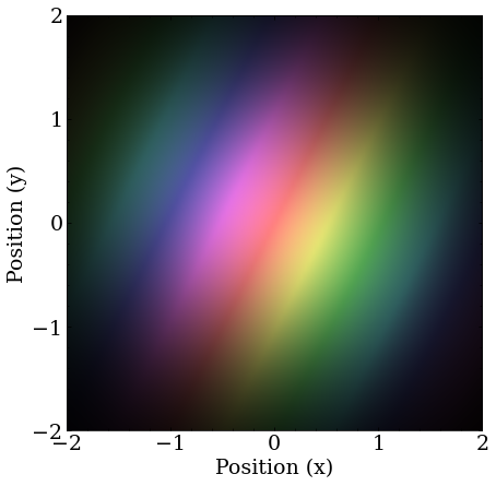
The initial guess for the Coulomb potential ground state search. There is slightly imbalanced momentum in the x-, y-directions, to break some degeneracy, and project onto a lot of eigenstates.
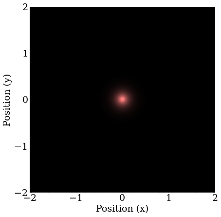
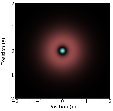
This evolves quickly (in complex time) to the ground state, which is the 2D analog of the orbital.
The final state, the orbital in 2D.
The next excited states are degenerate, meaning several states with the same energy, if one recalls the angular momentum states possible at higher energies . In 2D, the orbitals will be the same, and there will be and orbitals.
The first found is one of the orbitals, which is directed in the arbitrary direction of the momentum of the guess, because the guess projects more strongly on it than the other degenerate states.
Note that this takes a long (imaginary) time, because the only thing really splitting the degeneracy here is numerical error.
We find one of the orbital analogues in 2D. Let’s call it .
The second is the orbital quickly falls out after removing the momentum component, meaning this guess likely projects poorly onto the remaining orbital.
This is the orbital in 2D.
A very long time is required to stabilize on the final orbital, and the simulation spends most of it stuck on what looks like the 2D analogue of a orbital.
The result is the so-called orbital in 2D.
There’s even more degeneracy at the next energy level, and it would take a long time for this approach to converge, but in a real atom, there would be a magnetic field in addition to the electric potential, which would break this degeneracy by coupling to the orbital angular momentum of the electron. A project for another day, perhaps.
Update: I did write a follow up years later on simulating the double slit experiment, check it out!
>> Home