Introduction
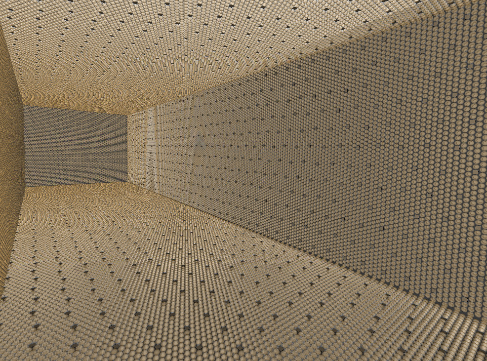
A Chroma model of the Theia25 detector with PMTs and LAPPDs as photon detectors.
Neutrino detectors like SNO+ and Theia don’t detect neutrinos directly. Instead they detect optical signals (light/photons) produced by high energy charged particles present after neutrinos interact in the medium. Detectors like these are typically large volumes (1 kt - 100 kt) of scintillating liquid for neutrinos to interact in (“target material”), and are surrounded by very sensitive light detectors to record the optical signals from the interaction. Scintillating liquids are preferred because they produce (relatively) large quantities of photons when charged particles move through them, and more photons means more information about the interaction.
This post will describe a method of analyzing these optical signals in order to reconstruct the position, time, and energy of the interactions in the detector. These quantities are the primary inputs to statistical analyses which tease out fundamental properties of neutrinos. I’ll give a brief overview of the physics of the interaction and detection mechanisms, and then jump right into reconstruction using both a traditional likelihood approach, and a (simplified) machine learning approach.
Physical interaction
The most common interaction detected is the elastic scatter of neutrinos off of electrons.
Because neutrinos only interact via the Weak force, these events are incredibly rare even though the number of neutrinos passing through the detector is very large.
Weak interactions happen when a neutrino exchanges a W or Z boson with an electron in the target material.
A particle physicist would represent this with the following Feynman diagram:
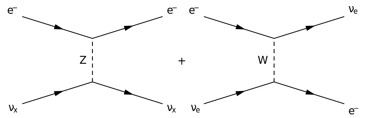 The left half represents a neutrino of any flavor ( with ) exchanging a neutral Z boson with an electron .
The right half is a similar interaction, but this time a charged W boson is exchanged, which converts electrons to electron flavor neutrinos (and the reverse) at each vertex in the diagram.
Both exchanges transfer energy and momentum from the neutrino to the electron.
Detected neutrinos, such as solar neutrinos, will have energies up to about MeV (mega electronvolts), and a large fraction of this will be transferred to the electron, which is essentially at rest compared to the neutrino.
This results in a high energy electron, with an energy and direction correlated with the initial neutrino energy and direction.
The left half represents a neutrino of any flavor ( with ) exchanging a neutral Z boson with an electron .
The right half is a similar interaction, but this time a charged W boson is exchanged, which converts electrons to electron flavor neutrinos (and the reverse) at each vertex in the diagram.
Both exchanges transfer energy and momentum from the neutrino to the electron.
Detected neutrinos, such as solar neutrinos, will have energies up to about MeV (mega electronvolts), and a large fraction of this will be transferred to the electron, which is essentially at rest compared to the neutrino.
This results in a high energy electron, with an energy and direction correlated with the initial neutrino energy and direction.
If the physical interactions make no sense, at some level the naive view of particle physics as tiny billiard balls colliding with each other applies here. Essentially, the “collision” is the exchange of a boson (compare to the Electromagnetic force exchanging photons), and the size of the objects being collided is proportional to the interaction strength. Compared to electromagnetic collisions that electrons usually participate in, where the apparent size (cross section) of an electron hitting another electron is around cm, the cross section of a neutrino hitting an electron is closer to cm. That’s a difference in size of twenty three orders of magnitude!
Optical photon production
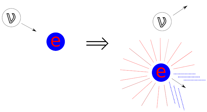 After the interaction, the neutrino continues on its way (a second interaction is incredibly improbable), but the now-highly-energetic electron is left in the detector.
As the electron moves through the target medium, it will slowly lose energy by colliding with other electrons.
This can ionize molecules, producing other free electrons, and can elevate electrons to higher energy levels within their molecules.
As these secondary electrons fall back to their ground state, photons are emitted with energy proportional to the difference in the energy levels, as scintillation light.
This light is emitted in random directions, depicted by the red rays in the diagram, but is highly localized to the path of the initial energetic electron.
After the interaction, the neutrino continues on its way (a second interaction is incredibly improbable), but the now-highly-energetic electron is left in the detector.
As the electron moves through the target medium, it will slowly lose energy by colliding with other electrons.
This can ionize molecules, producing other free electrons, and can elevate electrons to higher energy levels within their molecules.
As these secondary electrons fall back to their ground state, photons are emitted with energy proportional to the difference in the energy levels, as scintillation light.
This light is emitted in random directions, depicted by the red rays in the diagram, but is highly localized to the path of the initial energetic electron.
A Cherenkov ring detected in a simulated neutrino detector using dichroicons, which identifies Cherenkov photons by isolating long-wavelength photons.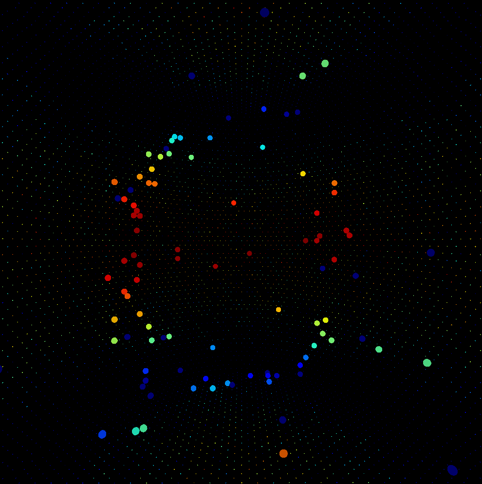
Photon detection
Compared to light you can see with your eyes ( photons/s), the light produced by neutrino interactions is relatively dim.
Scintillation light can deliver up to ten thousand () photons per MeV of energy, while Cherenkov light is 50 to 100 times dimmer.
A lot of this light is absorbed by the target material or other materials used in building the detector.
Therefore, very sensitive photon detectors are necessary to detect as many of the thousands of photons that remain.
Typically devices called photomultiplier tubes (PMTs) which utilize the photoelectric effect to absorb photons and emit an electron are used, since this process can occur with high fidelity.
These single electrons are amplified by accelerating them into metal plates in series, knocking out more electrons each time, until there is a detectable voltage pulse.
This allows PMTs to accurately measure single photons, and provide a measure of the time the photon was detected accurate to a few nanoseconds, which is a critical input for further analysis.
Below is a picture of the large area R7081 Hamamatsu PMTs used in the CHESS experiment I worked on at UC Berkeley.

The large area picosecond photodetector evaluated at UC Berkeley as an alternate light detection mechanism in the CHESS experiment.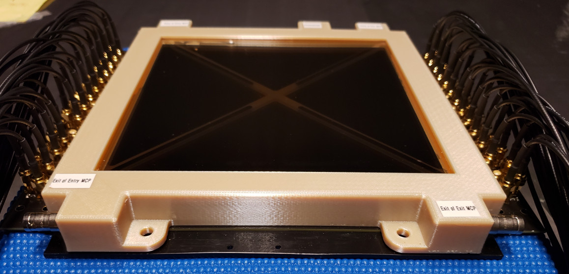
Reconstruction
Since these neutrino detectors only record the times at which photons produced in neutrino interactions are detected, there’s a considerable amount of work to be done to derive useful quantities from the data. The first step is to collect detected photons from the same interaction into single snapshots called “events.” This is usually quite easy, since all the photons arrive within a few hundred nanoseconds of each other, with relatively large time gaps between them. One must then recognize that these events are not always neutrino interactions. In fact most events are other things that might happen within a neutrino detector, including radioactive decay of trace elements, other physics like neutrinoless double beta decay, or just spurious flashes of light from high voltage arcs within the PMTs themselves. These different classes of events must be disentangled from the neutrino interactions. Fortunately, there are properties of these events which can be used to identify them, including where in the detector the event occurred, the time of the event, the energy deposited in the detector, the direction of the event, and the topology of the light detected from the event. Energy is simply proportional to the number of detected photons, though the proportionality constant is a function of the position in the detector, since the transparency of the target material and other optical effects will modify the probability of photons being detected. This means the position is one of the most critical quantities to reconstruct, and techniques for extracting these quantities are outlined in the following sections.
Likelihood method
The information available to reconstruction is the position and time at which photons labeled by the index were detected. If one assumes the photons were emitted all at the same time from the same point and travel with a velocity where is the refractive index, it would be relatively straightforward to determine the origin of the photons through the equation
which simply states that the travel time times the velocity is equal to the distance traveled. Each measured photon provides a separate which makes a solvable system of equations.
Reality is more complicated because there is uncertainty on both the detected position and time, and the photons are not emitted from the exact same positions at the exact same time. The former is a property of the photon detectors used, and these uncertainties can only be reduced with better photon detectors. The latter is a property of the particular path the high energy electron took through the medium, and the scintillation emission time profile, which can be large compared to the time the electron is actually moving through the target material. Further, not all photons move at the same speed, as the refractive index is a function of wavelength, resulting in rainbows, or more generally, dispersion, in optical materials, which spreads out the arrival times of photons of different wavelengths. Finally, photons do not necessarily travel in a straight line, as they could scatter or refract along the way. In general there is no way to know the exact path a photon took to arrive at a photon detector.
All is not lost, though, as several approximations can be made to make this problem tractable:
- The travel time is calculated assuming the refractive index for nm photons - a good assumption for Cherenkov and scintillation light detected by PMTs.
- Each photon is assumed to travel in a straight line from a single origin point - an approximation for sure, but vastly simplifies the problem from reality.
- Instead of assuming photons are all emitted at the same time, allow a time distribution that matches the scintillation time profile.
Using these approximations, define a quantity called the “hit time residual” that approximates the emission time of each detected photon:
The hit time residual distribution for a hypothetical neutrino detector. These show the time profiles of the different light sources: Cherenkov, scintillation, and reemission.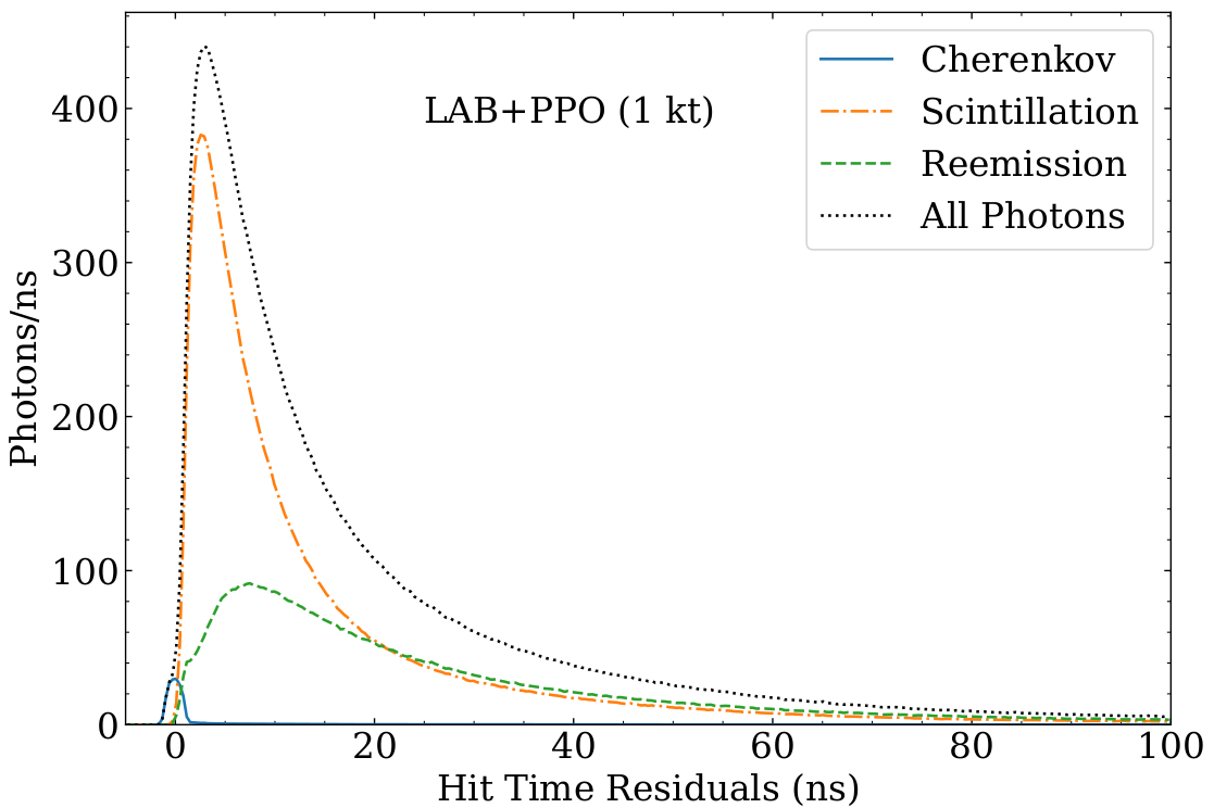
For any event where hit times and positions can be estimated (even with uncertainty), the likelihood can be parameterized as a function of the initial event position and time. It is then trivial to write a mathematical expression for the best estimate of the true initial event position and time:
Here, arg max is a bit of a cop out, since it means the arguments to the following function that result in its maximum value, which is not usually a trivial thing to arrive at. There are many variations on maximization (minimization) algorithms which can solve such a problem, but that’s a discussion for another time. Suffice to say, maximizing the likelihood here with a modern detector on the scale of tens of meters in size will result in few-cm and sub-ns resolution for the reconstructed neutrino event.
Machine learning method
Compared to a maximal likelihood method, which requires a lot of mathematical knowledge to implement a solution for a specific problem, machine learning with neural networks hides the detailed mathematical description of the problem within a generic framework for classifying data. The difficulty in extracting output parameters from data is offloaded into choosing a good encoding for the input and output and choosing a network topology that can learn to classify the data. In this case, the input data will be the the time at which each PMT detects its first photon, which is analogous to the from the likelihood method, except that we don’t need to tell the network where each PMT is, as the network can learn that. The output will be a representation of the position and time of the event.
Recurrent neural network structures, like the long short-term memory structure, have proven to be very successful at classifying time series data, and to leverage this structure, representing the input data as a time series is required.
For neural networks, a time series is data same shape that is sampled at different time slices.
For example, a single slice of the time series could be a series of values for each PMT with the quantity 1 (0) for PMTs that were (not) hit within that time slice.
In practice, I have found it better to weight the time slice before and after the PMT hit such that the weighted average of those two time slice times is the actual detected time.
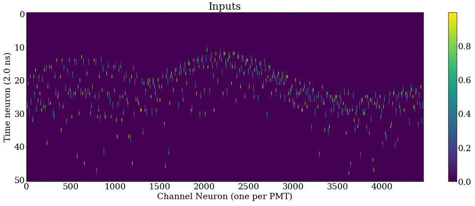
If these slices are stacked vertically, a 2D image is generated with axes of “PMT ID” and “time slice” is generated.
This is an accurate representation of the 2D tensor that is passed to the network as an input:
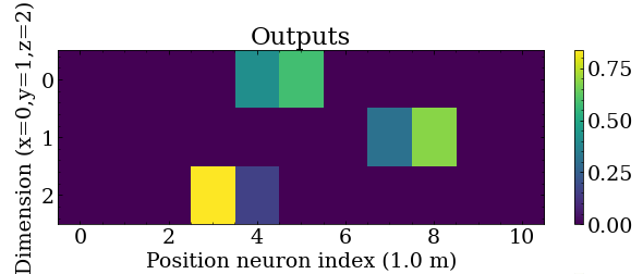
The output of this network will encode the true event position as a 2D tensor where one axis represents position slices and encode the true position similar to how time is encoded above, and the other axis represents X, Y, or Z dimensions.
For example, to encode the X position, the two neurons in the X dimension row nearest the true X position are weighted such that the weighted average is the true position.
This could easily be three separate 1D output tensors, however since the dimensions are encoded the same way (11 neurons at 1 meter spacing) it is possible to use a single 2D tensor:
The network topology was implemented using Keras (tensorflow) and is as follows:
- 2D input tensor with the PMT time series
- LSTM with 256-length output which digests this timeseries
- 256-length hidden state is fed into a 256-length fully connected dense layer
- A 33-length fully connected dense layer, that is reshaped into a (3,11) tensor where the first dimension is the axis, while the second dimension encodes the offset in that axis.
The code to generate this network (along with additional code to reconstruct direction, which I may get into in a different post) can be found here:
# Very simple proof of concept network topology
# timesteps x channels input series
# 256-neuron LSTM with final hidden state output
# Dense neuron layer for each output dimension (xyz,theta,phi)

time_series = layers.Input((None,num_channels),name='time_series')
lstm_h = layers.LSTM(256,name='lstm')(time_series)
state = layers.Dense(256,activation='tanh',name='state')(lstm_h)
activation = 'sigmoid'
pos_out = layers.Dense((3*pos_bins),activation=activation,name='pos_intermediate')(state)
pos_out = tf.reshape(pos_out,(-1,3,pos_bins),name='pos')
theta_out = layers.Dense(theta_bins,activation=activation,name='theta')(state)
phi_out = layers.Dense(phi_bins,activation=activation,name='phi')(state)
model = keras.Model(inputs=dict(time_series=time_series),
                    outputs=dict(pos=pos_out,theta=theta_out,phi=phi_out),
                    name='PositionDirection')
model.compile(optimizer='adam',loss='mean_squared_error')
Because the input to this network is large, this network contains roughly 4 million trainable parameters. The network is trained on simulated events (as depicted above) where the initial position is known. It can then be used to reconstruct events it has never seen. This reconstruction is done by weighting the positions represented in the output neurons by the activation of the neurons. This procedure results in a comparable position resolution to the maximum likelihood method above.
Where to go from here
With the position (and time) known, there are still other quantities that could be reconstructed, such as the direction of the event if the Cherenkov photons can be identified. After this, PDFs as a function of the reconstructed quantities are generated for each class of event that may be present in the dataset. Finally, a maximum likelihood method not dissimilar to the position reconstruction method used above is employed to determine the number of each type of event in the dataset. The relative frequency of certain classes of events, or simply the (non)presence of a certain class of event, can be a physically meaningful result. For instance, the SNO detector measured the distribution of neutrino flavor from solar neutrinos to solve the solar neutrino problem while the upgrade of SNO, SNO+, aims to set an upper limit on the rate of neutrinoless double beta decay by demonstrating that there is always energy carried away by neutrinos in isotopes that undergo double beta decay.
>> Home