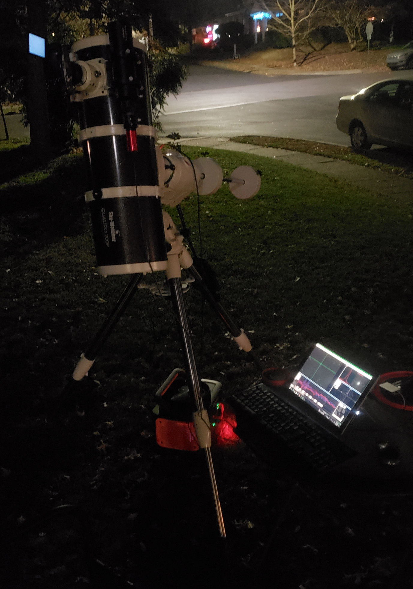
I’m now the proud owner of a Sky Watcher Quattro 200P on a EQ6-R Pro mount. Currently paired with a Sony α7C and coma corrector, along with the occasional OSC filter. Guiding to 0.6" with a ZWO ASI120MM on a Svbony 60mm F/4 106SV guide scope. Living the dream.
Now that I have a nice astrophotography setup, I’ll consider doing a series of posts for completed targets. At the moment, I’ve simply got a shared album with the results and a bit of target info in the descriptions for the various deep sky objects I’ve imaged. Deep sky here means that these objects are typically thousands (nebulae) to tens/hundreds of millions (galaxies) of light years away. Despite being so far away, these objects are often quite large in the sky, ranging from minutes to degrees in the night sky. Common in astronomy, a minute, or more properly an arcminute, is 1/60th of a degree, with an (arc)second being 1/60th of an (arc)minute. The moon is aroud 30’ (thirty minutes) across when full, for a sense of scale.
The further I go in this hobby, it occurs to me that people don’t generally understand what they’re looking at when they see a deep sky photo. Even in perfectly dark skies, with a really good telescope, one doesn’t see much with a telescope besides shades of darkness for most objects, if anything is visible at all. What’s more, being closer wouldn’t improve the situation much, by eye. These objects are very faint, and displaying them requires very long exposures to make precise measurements of differing levels of faintness.
Turns out, this process works nearly as well in heavily light polluted areas as it does in dark sky areas, given enough time. My work, for instance, is primarily from Bortle 7. The rest of this post will detail the technique in general, and various offshoot practices.
Imaging from a mathematical perspective
An image as collected by a modern digital sensor is a collection of light intensity measurements at many individual pixels. Combined with an optical system, each pixel on a sensor becomes a measurement of the intensity of light in a particular direction with respect to some viewer. Typically these pixels are on a two dimensional grid, so one might say an image is made of pixels for a grid-like collection of slices of the sky .
Physically, photons from a particular direction are focused onto a pixel of some imaging device and converted into some measurable signal, with the reported value being nominally proportional to the number of photons. The absorption of photons would be a Poisson random process from any number of different sources in that particular direction . Let’s categorize the rates of those sources as signal of the deep sky object we want and background such as light polution or skyglow. That means the total photons asorbed in a pixel, , for a span of time is given by
where the is a pixel-depdendent efficiency to convert photons to signal. The value reported for the pixel would include a gaussian random error with a mean of and standard deviation of a few photons (typically) due to electronics bias and noise, respectively.
This is technically just a mathematical model, but is well motivated by how both CCD and CMOS digital sensors work, along with any other technology that would be based on counting photons.
If we look at the expectation value for a pixel, we find the obvious result that after infinite measurements, the pixel will limit to be proportional to the signal plus background by the exposure time
perhaps with the surprise that a bias error shows up. For most sensors, this bias is small compared to light levels usually encountered, but may not be insignificant if the integration time is small or the signal is particularly weak for a deep sky object.
The variance is simply,
meaning the standard deviation, or uncertainty,
doubles down on the need for good exposure: maximize such that the electronics noise contribtuion is not dominant.
Uncertainty reduction through averaging
Notable here, due to the nature of counting a Poisson process, is that the uncertainty in the photon sources are proportional to the square root of the photon signals. This means the uncertainty actually is larger for longer exposure times. Fortunately, as it only grows with a square root, all is made well again with some averaging. If there are measurements of , the expectation of the sum is
making the average of measurements
which seems a bit tautological, until you check the standard deviation of the average of measurements,
where the fact that uncorrelated variances add was leveraged to pull out the factor. This immediately reveals that the average of many images multiplies the uncertainty at any pixel by a factor of compared to a single image, meaning there are diminishing returns to averaging more images (must double the quantity averaged for the same factor of uncertainty reduction) though the uncertainty continues to decrease.
Precision signal extraction
Unfortunately, what we really want is an image of just the exposed signal . If we take for granted that there is a method to estimate the average background contribution at a pixel
and that the electronics bias is a fixed, measurable effect, meaning that is known, we can define a new image based off the old one as
This new image has an expectation value of
with the background and bias removed, as designed.
The standard deviation, however, remains unchanged
since we have only subtracted constants off the pixel values, which are random variables here.
With enough averaged measurements, ultimately this standard deviation will decrease to zero, but it also highlights the aspects of imagaging to optimize for quality, which can be more clearly seen in the ratio of the uncertainty to the expectation value.
With the intuition that the uncertainty should be small relative to the desired value, some observations can be made:
- It is important to have high detection efficiency and long exposure times for combatting electronics noise.
- The same combination minimizes the number of images needed for the same quality, even if electronics noise is insignificant
- The larger the ratio of the backgound to the signal, the more difficult the measurement will be.
- More precisely, a signal that is times dimmer will require roughly times more images to achieve the same uncertainty.
A full calibration technique
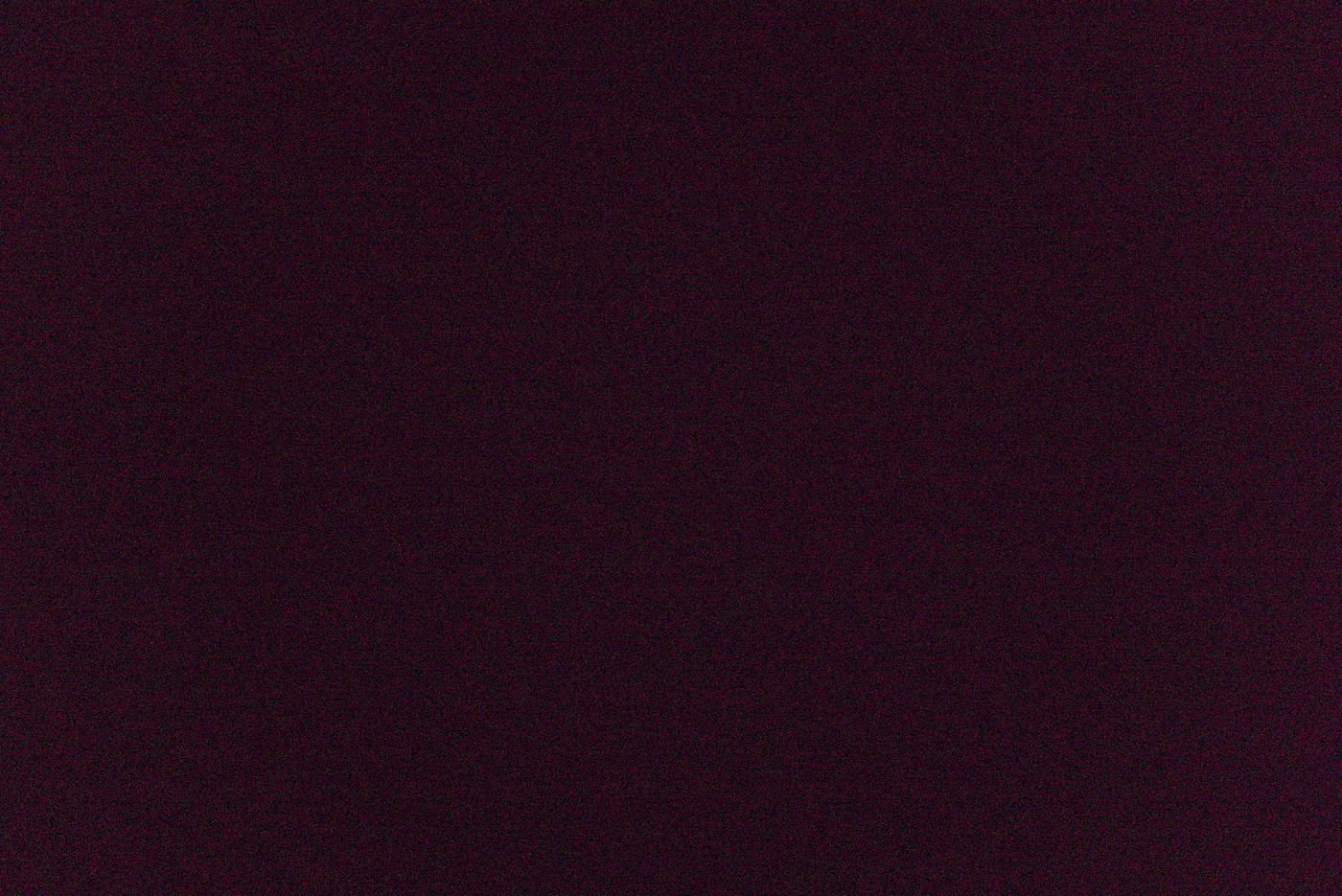
A 30s exposure light frame with my Tamron 70-300mm @ 300mm F/9 ISO 2000 pointed at M31 the Andromeda Galaxy. A dark frame, boosted 6 stops to allow something other than dark to be seen. My Sony α7C has very low dark counts. A flat frame from the Andromeda session that provided the light frame above. A bias frame, boosted 6 stops to allow something other than dark to be seen. Almost no bias on these excellent CMOS sensors.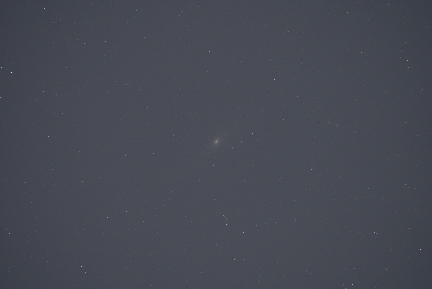


Knowing the detection efficiency it is possible to define the desired calibrated signal image to be extracted from the measured values coming out of the camera, the latter being called lights in the astrophotography community.
where
and
which doesn’t modify the analysis of uncertainty at all.
In this formalizm, corresponds to the calibration information gained from flats, to darks (or biases depending on context), and to a background estimation technique, to borrow more terms commonly used in astrophotography.
Flats for detection efficiency
Obtaining flats typically requires imaging something that is known to be uniform (signal only, no backround), such that the uniform assumption can be used to back out the for each pixel. Many images are taken to reduce uncertainty in this calculation, however bias in the flats must be removed from the pixels, as it won’t average out with repeated measurement. Often, very short images minimizing are captured, such that the pixels are dominated by whatever bias might exist, and this is directly used as the bias.
This is all well and good, as long as the flat images themselves don’t contain any other kinds of bias than those captured by minimal exposure time. I note in the next section that the differences between darks and biases as usually referenced is that one is used for the bias calculation of lights and the other for flats. I assert the same technique should be applied in both cases, with the exception being that the bias picked up by darks would include effects from the very long exposure times of the lights while the likely shorter exposure times of the flats may get away with very very short bias frames.
Darks for bias
Colloquially called darks to differentiate from the biases used in producing the detection efficiency, the images usually referred to as darks are in fact just the bias calibration data for lights. I’ve treated as something indepdent of exposure time (and therefore achievable at 0 exposure time) as mentioned in the last section, however the community strongly recommends taking darks at the same exposure settings as lights. The reason for this is effects like “amp glow” act like a bias in that they don’t average out, but rather build up over the exposure time. Biases are taken with no visible signal or background such that is the only term present in the pixel readout.
Background extraction
After calibrating the bias and detection efficiency, all that should be left in the result of processing one of the light frames is an image with values proportional to real light, be it signal or background. It is common in this situation to make assumptions about what the background light might look like, i.e. if it is primarily light pollution, it should be very uniform across the small patch of sky being immaged. By judiciously choosing points within the image consisting primarily of background, an average measure of the background for the entire image could be calculated and used for the values. Some other functional form for the background could be fit in an analogous method to derive the bias calibration.
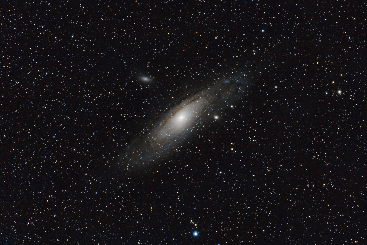
The final calibrated and stacked image of Andromeda with my Tamron telephoto zoom lens, utilizing Siril for calibration processing, alignment, stacking, and stretching.
Calibrated astrophotography
The calibration technique described above requires flats, biases, and darks to go along with the lights containing the signal and background. It’s important to note that each italicized word is a collection of images to reduce variance to acceptable levels. The quantity of each light and dark set is related to the ratio of the background light pollution to the target deep sky object’s light signal. The darks are linked to the lights as the direct subtraction of the two means the variance in the result will be at least the larger of the two. The divided-out flats and their biases contribute similarly, but are typically much faster to take, requiring much less exposure time for the same variance.
Detection efficency is extracted from flats and biases, which constitutes both the pixel’s sensitivity and any inefficiencies (dust, relative, or otherwise) in the optical system. Bias and associated effects with nonzero expectation values are captured in the darks. By calibrating these effects, and taking enough data to reduce variance to below the signal level, background extraction can be done successfully, resulting in a nice image of a deep sky object, even under heavy light pollution.
Technically, without these calibrations, a long exposure image is likely to be dominated by the errors that would be calibrated away. Taking all of this additional data can be a chore, especially since the only signal data is present in the lights. Thankfully, there’s an alternative solution.
Dithering instead of calibrating
Up to now I’ve assumed that every exposure of a slice of the sky would correspond to the same sensor pixel each time. If instead slightly misalign the position or direction of the sensor such that a random pixel captured the light from the slice of sky , things change a bit. Namely, the pixel-specific calibration values for that slice of sky take on a distribution corresponding to the properties of the sensor. If we assume enough samples are taken, we can assume the pixels have approximately Gaussian distributions for their properties. This is not especially true for the detection efficiency which is strongly position dependent compared to the scale of intentional misalignment, but we’ll come back to that.
Now the expectation value for the measurements of that slice of sky can be written in these terms,
revealing that only the average bias of the sensor and average detection efficiency (more on this) need be known to calibrate a sufficient number of randomly shifted frames.
The process of randomly adjusting the position a bit is called dithering in the astrophotography community, and is now exclusively how I take images. How true these assumptions are (how well dithering can replace proper calibration) depend on how uniform your camera sensor is compared to the scale of the dirthering perturbations. For example, if your camera is covered in dust shadows, but every perturbation is very likely to move a totally random set of pixels into a dust shadow, the dust won’t show up in the final stacked image. Similarly, if the bias variation is well sampled, this ends up being very simple to remove with a linear black point calibration in the final stacked image.
Detection efficiency, largely due to vignetting from the optical system, typically varies on a scale larger than dithering. The pixel-to-pixel effects, and effects like dust, will be averaged out, but the vignetting will likely remain unless the dithering step is comparable to the size of the frame. While possible in mosaics, such a large dithering step size would waste considerable time on smaller targets. Small dithering will still smooth this effect out, however, and I find that the resulting stacked images have simple consistent, radial profiles that can be removed with a functional form background extraction, like the RBF method.
With that in mind, my post-processing technique for stacked, dithered images is to:
- Subtract off the bias with a black point adjustment.
- Utilize the RBF method to divide out the vignetting, obtaining a flat background.
- Subtract off the flat background with a final black point adjustment.
Following that, I’ll do a bit of color calibration with stars of known temperature, and send it out into the world.
Of course, you could dither and calibrate for even further variance reduction, no one is stopping you… I just don’t find the calibration data particularly enjoyable to take.
Update 2025-12-30: Dither and take the calibration data, its worth it! Dithering still helps correct for things that slip past calibration, but dithering and background extraction destroy dim targets on uncalibrated data. This and other learnings after some years of experience can be found in a future post on high quality images
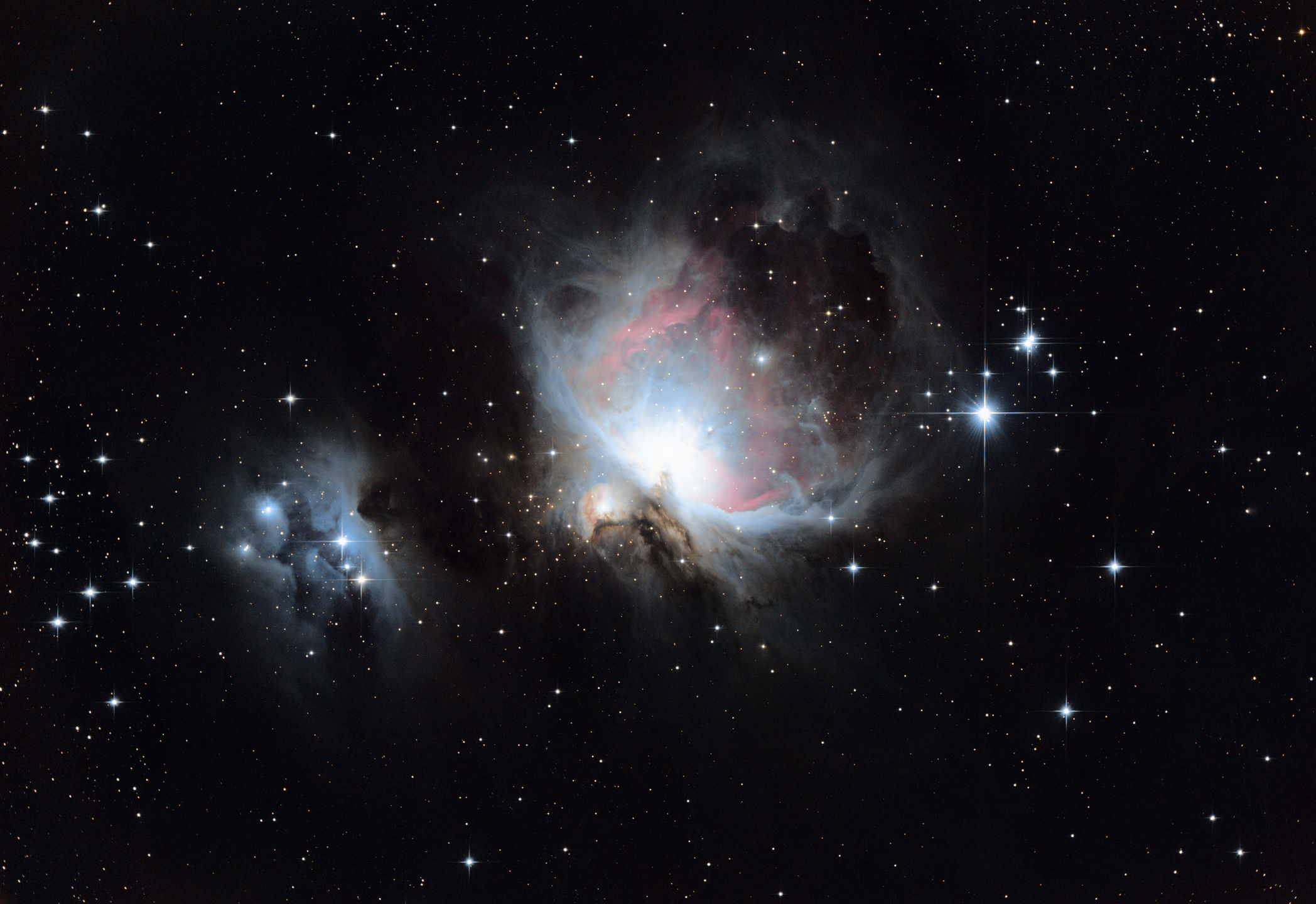
M42 the Orion Nebula - dithered, stacked, and processed with no other calibration data. This one was taken with the real telescope, not a camera lens as the earlier images were.