This post will try to give a grounded conceptual (with a side of mathematical) understanding of quantum computing by comparing it to classical computing. This can be a bit tricky, since robust quantum computers are still a nascent technology, but I’ll stick to the low level concepts here instead of getting into the esoteric science that is programming quantum computers. Primarily I want to motivate why quantum computing is fundamentally different from classical computing, and how it is the same.
Representation of information
Classical bits, like those used in your computer, can be in one of two states: high () or low (). These are physically realized as toggle switches for electrical current (specifically flip-flops), which are literally in an on or off state. The possibility of exactly two discrete states per bit means that collections of bits are able to represent discrete configurations. Operations can be represented as functions that map from one configuration of bits to another. Algorithms can be constructed as collections of operations in particular orders. Around this, all of modern computing has developed.
Single Qubits
Quantum bits – qubits – are two state quantum systems. These are physically realized in many ways, and two common examples are the spin of an electron or polarization of a photon. The difference between a classical bit with two classical states and a qubit with two quantum states is that quantum mechanics is probabilistic, and describing how a two state system behaves physically requires a careful accounting of all possibilities. All possibilities includes any arbitrary mixture of the possible outcomes, which means observing a qubit in one of its two states. Observing it in a particular basis state, either or , could happen all of the time, none of the the time, or some mixture. Rigorous physical and mathematical treatment of an arbitrary two-state system, , reveals that the two states can be thought of as being mixed together with complex coefficients:
Classically, that is when the state is measured, is found to be either or in any particular instance. On the other hand, as long as the two state system is left isolated or carefully controlled, it will evolve into very interesting combinations of or with real and imaginary components.
The physical interpretation of this formalism is that magnitude squared of the complex components is interpreted as a probability to be measured in the particular basis state . So, by performing many experiments that result in the same and measuring the distributions of to , the relative magnitudes of and can be determined, and there are similar operations to determine the relative phase.
Some mathematical formalism
Mathematicians would say this combination of two basis states spans a complex Hilbert space, meaning that the two states are like two axes in a world where the coordinate axes are complex numbers, and the state is a point in that 2D space. This is a form of abstract vector space, and the the arbitrary state is often called a state vector in physics for this reason. Most of the intuition from normal vectors in linear algebra will carry over to state vectors. Along these lines, one could write as a column vector.
The probabilistic interpretation of the magnitude squared of the components implies that the sum of the magnitudes squared of all , or the magnitude of the state vector, should be . Thinking about this from the perspective of an inner product (or dot product), which computes the magnitude squared of all components of a vector, this means something like the probability of a state to be itself is 100%.
This idea of a state being another state in abstract vector spaces is captured by a more rigorous definition of the inner (or dot product, from linear algebra). The inner product of the state with itself is historically written as :
This introduces the idea of a conjugate vector which flips the sign of the imaginary part of all the complex numbers (flips across the real axis – conjugation is denoted with ).
A conjugate vector like this would be written out as a row vector instead of a column vector
and normal matrix multiplication would provide the result.
In the notation of physics one needs to understand that the two basis states are distinct in the sense that their inner product is zero, while the inner product of a labeled state with itself is unity. All other usual linear algebra rules apply.
So, probability of the particle being in its own state being 1 means the coefficients are subject to the constraint:
which puts decent constraints on the magnitudes of the two coefficients, such that one fully determines the other, but does not strongly constrain the phase.
Back to the implications

The Bloch sphere represents the space of possible states for a 2-state quantum mechanical system, paramaterized by and for the generic state .
Typically only the relative phase of the two states is physically observable, leaving the relative phase and relative magnitude as the only free parameters here, even though a state is represented by two complex numbers (four real numbers). Often these two remaining parameters are thought of as the surface of a sphere, where the latitude is the relative magnitude (poles being purely one or the other state) and the relative angle being the longitude.
In simpler terms, this means one qubit can represent a point on the surface of a sphere, which is clearly quite a bit more information than simply “on” or “off”.
Multiple Qubits
The true power comes when one considers collections of two-state systems, or collections of qubits called quantum registers. Separately, qubits are two-state systems, but considered together (which brings some serious engineering challenges) they are much more, because any measurement outcome now has possibilities, and the probabilities of each must be correctly accounted for.
For a two qubit system, we get combinations of basis states from both qubits like representing the zero state of qubit 0 and qubit 1, which is often written as just letting the index of the digit define the qubit the digit is for. All the possible outcomes of a 2-qubit system are:
The treatment above finds the 2-qubit 4-state system has three free relative phases and three freely determined magnitudes, meaning six free parameters. For 3-qubits we have:
7 relative angles and 7 magnitudes; 14 parameters. This grows exponentially with the number of qubits!
The salient point here is that for quantum registers, the number of free, real, parameters is for qubits. This is often misquoted (and I will below) as , as it is approximately that for large , and because it takes complex numbers (which are inherently two-dimensional, with a real and imaginary part) to specify a point in the dimensional complex Hilbert space of a -qubit register.
Extreme information processing density
The above means an -qubit quantum register is represented by a state of approximately real-valued parameters while classical registers can only represent one of unique values for bits.
While each operation on classical register can result in one of results, contingent on some algorithm with possible inputs, an operation on a quantum register can result in real values contingent on some algorithm with real value inputs. This means a 32-qubit quantum computer could - in theory - operate on around eight billion real numbers at once - a feat that your average 32-bit classical computer would require around eight billion operations to accomplish, assuming those real numbers could be approximated by 32-bit floats. Pushing this to larger numbers of qubits – say, 64 – reveals computational power unparalleled: nearly 10^20 state values operated on, which would take a modern 64-bit processor core thousands of years to simulate, if the thousand exabytes of RAM needed to hold the state existed.
The idea of operation on large batches of real values at once is what makes quantum computing attractive. This massive parallelism has inspired algorithms to factor very large numbers quickly, there are clear applications to neural networks, and even more mundane things like rapidly multiplying matrices can be done. However, while one can imagine how a classical switch might be turned off and on to represent a bit used in computations, operating on a qubit - or quantum register - is far less easy to imagine. With that in mind, I’ll try to show here a comparison of foundational quantum computing concepts to those that underpin modern classical computers.
Basic architecture
Modern computers are based on tiny electrically operated switches, called transistors. These devices exploit the fact that the conductivity of interfaces of certain materials known as semiconductors can be changed by orders of magnitude with application of electrical potential in the right place, allowing them to conduct or not depending on whether some upstream switch is conducting or not. Combining transistors with resistors allows for the construction of logical gates which have well defined rules for how the output behaves given some input. These rules are simple maps from a discrete set of input configurations to a discrete set of output configurations, called a logic table.
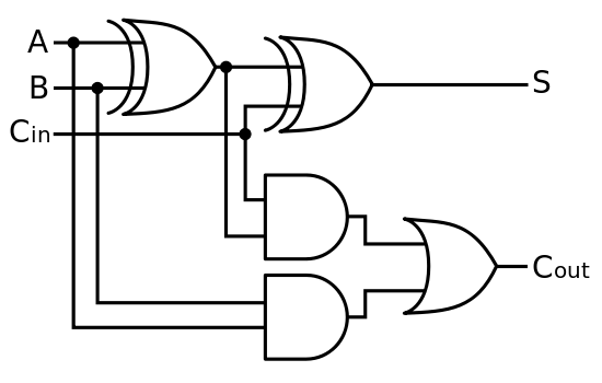
A full adder can be chained together into a circuit to add registers of classical bits representing integer numbers. From top to bottom, XOR, AND, and OR gates are used.
Combinations of logical gates are used to implement particular operations on collections of bits, like this full adder in the circuit diagram to the right. Each symbol refers to a particular logic table to control the output, and the lines refer to how the tables outputs are used as inputs to other tables. By building up more and more complicated circuits, a library of common operations is created, from which any other operation can be efficiently constructed. Computer programs are then written to choose the order in which these operations are applied and to which collections of bits, to implement classical algorithms that allow your computer to do interesting things. Given enough time and bits, these algorithms can solve almost any problem.
Quantum computation
Quantum computers instead use physical phenomenon like the spin of an electron as their base unit of information. These spins can be manipulated with electromagnetic fields (external or other qubits) to perform operations, or be kept in isolation to store quantum information. The exact details of moving quantum information around and holding it for long timescales are the limiting factor for practical quantum computing in 2023.
The physical idea goes like this —
- External stimuli can be used to put a system of qubits into some known state
- A series of operations can do something useful, like perform some calculation.
- Finally, the result can be measured.
By repeatedly performing the same quantum calculation over and over and measuring the result, the configuration of the free parameters at the end (the result of the calculation) can be determined.
I’ve said that physical qubits can be manipulated with physical interactions like magnetic fields, but exactly how this translates into computations merits some further explanation. From a computational perspective, we have the following analogy.
- Classical A circuit represents some operation by mapping a particular configuration of bits to some other configuration of bits according to the rules of that operation.
- Quantum A contrived physical situation represents some operation by causing a physical state to change in a certain way into another physical state according to the rules of that operation.
In other words, an operation is something that causes an arbitrary state to change into some other state . This is accomplished by arranging the physical environment (turning on a magnetic field, in a particular direction, for a particular time, for instance) the qubits are in such that the normal quantum mechanical evolution of the state proceeds in a certain desired way. To double down, compare this to arranging transistors and resistors in a certain way such that the flow of electrical current goes in a certain desired way. Both scinareos can be used to compute, but the quantum one has access to a much larger space for operations.
Quantum operations
Describing how to change an arbitrary state into another state means understanding how states change in the first place. Borrowing from the mathematical formalism earlier, we know that any state can be described as a vector of complex coefficients with unit magnitude. It is known that the most general type of operation that transforms a unit complex vector into another complex unit vector is a complex square matrix with the unitary property. More specifically, if the state vector has components, then an arbitrary operation can be represented by the operator which is an matrix that preserves the length of any vector it operates on.
Transformation of a state by an operator is written like
It is important to note that not all possible operators are easy to implement physically, but there are a collection of operations that are sufficient to construct many useful algorithms. This is analogous to how there are many possible classical logic tables, but only a finite set of simple ones (AND, OR, NOT, XOR, etc) are necessary to perform any calculation.
To make this a bit more concrete, consider the quantum equivalent of the classical NOT gate, which inverts the inputs, often called . For a single qubit, takes the matrix form
meaning that it swaps the coefficients of the two states, much like NOT swaps the logic level of the input.
It is called the gate, because it represents a 180-degree rotation around the X-axis of a Bloch sphere, which can be physically realized by applying a certain frequency of electromagnetic radiation for a certain amount of time to the qubit in question.
Deep into the math of Quantum Mechanics
Ultimately the dynamics of any quantum system are governed by the Schrodinger equation, and this is no exception. The unitary operators here can be derived from a Schrodinger equation for a particular Hamiltonian and potential, and often that is the more convenient perspective to consider when trying to physically realize quantum logic gates.
Diving into the math of quantum mechanics, but this time with matrix instead of wave mechanics, one can design a Hamiltonian operator on the state vector such that the energy of the state is given by
Then the solution to the Schrodinger equation,
which governs time evolution, is
which is manifestly true, as long as you don’t think too hard about what raised to the power of a complex matrix is!
As it turns out, if is an eigenstate of the Hamiltonian, this is the usual result that energy eigenstates only change phase in time. In a two-state system, if both basis states are eigenstates have the same energy, both states will stay in phase as time moves on, and this would correspond to an identity gate in the quantum logic gate world.
If both basis states are eigenstates with different energies, with separation , this would correspond to a phase shift gate, where the amount of phase shift would depend on the amount of evolution time.
Recall that in both cases, the overall phase is not observable.
When is not an eigenstate, things are a bit more interesting, and the unitary matrix representing evolution under the Hamiltonian for some time is given by
which can be understood as the series expansion of the exponential function to be
with a matrix raised to a power meaning repeated application of that matrix.
In this way, the unitary operators that describe quantum logic gates can be assumed to be given by time evolution of the Schrodinger equation for particular physical scinareos.
Universal Computation
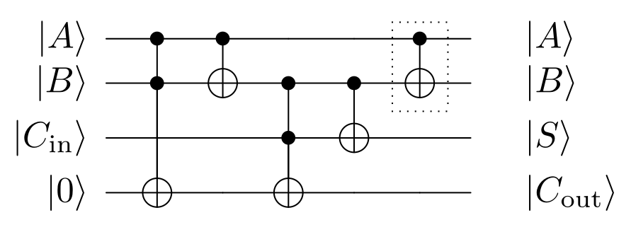
A quantum full adder can be chained together into a circuit to add registers of quantum bits representing superpositions of integer numbers. Triffoli and CNOT gates are used.
A set of operations, often called quantum logic gates, are known to exist, which can construct any (with few caveats) quantum operation. The list is not huge: , , , , , , , , , and Toffoli () are common, and physical implementations exist. This allows quantum circuits, like the quantum full adder to the right, to be constructed to do useful computations. Like the classical scenario, these can be built up into vastly complex operations in aggregate.
Practical Quantum Computing
In much the same way that you would not write a computer program by selecting transistors and resistors and wiring them into logic gates to build up your program, quantum computing nominally does not involve thinking about the detailed construction of the quantum gates. There would be some “quantum compiler” which translates or compiles a language based on quantum concepts into a plan for applying operations (quantum gates) to particular quantum registers. There are Python packages like Qiskit which even supports targeting backends with different “instruction sets” (quantum gates) available. Indeed “machine code” for a quantum computer like QASM has existed for a while, and can describe any quantum algorithm as long as the hardware implements a universal set of gates.
In this way, a quantum computer could be used similar to a modern classical computer, in a way that leverages a finite set of pre-engineered operations from which any arbitrary quantum program could be constructed. That’s the theory, anyway, and offerings like IBM Quantum are well on their way to commercializing it!
>> Home