Photon simulations for DUNE
The DUNE experiment is nominally a time projection chamber (TPC), which records the paths of high energy charged particles by collecting the ionized electrons left in their wake. Studying the paths of these particles gives information on the particular type of physical interaction responsible for creating them. DUNE is particularly interested in the particles produced by neutrino interactions, and will be constructed in a high intensity neutrino beam to make those interactions much more common. The energy deposited by the high energy particles as they travel through the liquid argon does more than just ionize the argon atoms, it also produces scintillation and Cherenkov light. These optical signals can provide complimentary information to the tracks from the TPC, and are especially interesting for lower energy physics, like solar neutrino interactions.
DUNE plans to include optical detectors sensitive to the short wavelength (128nm) argon scintillation light, called ARAPUCAs. Before construction, the ideal placement and expected impact of the ARAPUCAs on the physics program of DUNE in various detector geometries must be understood. To understand how photons produced in the physical interactions arrive at the ARAPUCAs, a full optical simulation of the DUNE detector is the ideal. This is a task that is well suited for Chroma, a fast GPU-accelerated photon simulation that I have worked with the past several years.
GDML geometries
The largest difficulty, besides integrating Chroma into the DUNE simulation software, is to provide Chroma with an accurate model of the proposed detector geometries. DUNE has heavily invested in the Geometry Description Markup Language (GDML) for describing its detector geometries, and has many iterations of geometries to consider. GDML is essentially an XML file that specifies the structure of a geometry used by Geant4 for particle physics simulations. It uses a common technique to define complicated shapes as boolean operations on simpler shapes, creating what is known as a constructive solid geometry (CSG). Many CSG shapes are specified to be placed at particular positions and rotations within a 3D space, and these spaces can then be nested to form very complex geometries. Each placed CSG shape is also associated with some material properties, so that the physics simulation can accurately propagate particles through this simulated world.
On the other hand, Chroma typically works with triangular meshes as the basic unit of geometry, and places these triangular meshes at arbitrary positions and locations within a world. This is a very general technique, since arbitrary triangular meshes can be generated by CAD programs like SolveSpace and then imported into Chroma. Unfortunately, to my knowledge, there was no out-of-the-box solution for automatically converting a GDML’s CSG structure into triangle meshes, since GDML is a very niche format used almost exclusively by particle physics. Since there are many DUNE GDML files, with the promise of more in the future, converting by hand was an exercise in futility. So, I decided to write a GDML parser and use the CSG information to build triangular meshes for Chroma from scratch, which can be found in the Chroma repository, and is described below.
A Chroma GDML importer
GDML files, fortunately, are standard XML and not some niche format for which only one parser in one language exists (looking at you, fhicl). This means throwing together something to parser a GDML file into something one can manipulate symbolically in Python is as simple as
import xml.etree.ElementTree as et
xml = et.parse('geometry.gdml')
A glance at a GDML file in plaintext indicates the structure is fairly intuitive, and I’ll state for the record that I never actually looked at any proper documentation on the GDML format because I couldn’t find any after a few google searches. The concepts follow the geometry mechanisms of Geant4 very closely, though, so I had enough experience to tease out the details. A simplified sketch leaving off many attributes is shown here.
<gdml>
  <define>
    <!-- position and rotation constants -->
  </define>
  <materials>
    <!-- material properties -->
  </materials>
  <solids>
    <!--CSG definitions -->
  </solids>
  <structure>
    <!--volumes (containing solids) definitions -->
  </structure>
  <setup>
    <world ref="some_volume" />
  </setup>
</gdml>
For Chroma, the three most important tags are define, solids, and structure, with the setup tag simply specifying which of the volumes in structure is the outermost volume (the “world” in particle-physics-simulation lingo).
GDML makes use of named references throughout, where a ref will be specified that is an implicit match to some tag with a name attribute whose value matches the ref.
This is used frequently for positions and rotations, which appear under the define tag.
<position name="posCenter" unit="cm" x="0" y="0" z="0"/>
<rotation name="rIdentity" unit="deg" x="0" y="0" z="0"/>
The fields with numbers can apparently have math in them (e.g. "1+2" evaluates to 3), so some calls to Python’s eval is critical here.
Some slides I found discussing GDML suggests that constants can also be defined in this define section, and those constants can be used as variables in math attributes, but the DUNE GDML files do not use this functionality, so I have not considered it yet.
Python’s eval does support passing a dict with the global scope, so this would be trivial to handle, if needed.
Mesh construction
The CSG geometry is easily the most difficult part of this, but a general solution is as easy as exploiting the PyMesh package, which provides a nice Python interface to state-of-the-art CSG toolkits.
For example, everything in DUNE geometries use the primitive box and tube shapes as the base objects in its CSG solids.
These appear as named tags under the solids tag, and I defer to Geant4 documentation for understanding the meaning of the attributes.
<box name="Inner" lunit="cm"
  x="360.843"
  y="607.82875"
  z="232.39"/>
<tube name="InnerWireU0"
  rmax="0.0075"
  z="1.28356534760138"
  deltaphi="360"
  aunit="deg"
  lunit="cm"/>
And, after parsing, can be constructed as PyMesh meshes.
def box(x,y,z):
    '''Generate a mesh for a GDML box primitive'''
    return pymesh.generate_box_mesh([-x/2,-y/2,-z/2],[x/2,y/2,z/2])

def tube(z,r,segs=None):
    '''Generate a mesh for a GDML tube primitive. Note: does not support all Geant4 parameters.'''
    if segs is None:
        segs = max(9,int(r*16))
    return pymesh.generate_cylinder([0,0,-z/2],[0,0,+z/2],r,r,num_segments=segs)
To create more complicated shapes, DUNE exclusively uses boolean subtraction, which also appear as named tags under solids.
<subtraction name="APAFrameYSide">
  <first  ref="APAFrameYSideShell"/>
  <second ref="APAFrameYSideHollow"/>
  <positionref ref="posCenter"/>
  <rotationref ref="rIdentity"/>
</subtraction>
Here, first and second are sub tags instead of attributes, for some reason, and specify solids by name using the ref attribute.
second is subtracted from first after an arbitrary position and rotation.
Here, position and rotation are specified by reference, but I suspect that position and rotation tags could be used here, so implemented the ability to parse either.
PyMesh then implements the boolean operations, and could easily be extended to perform more than subtraction.
a = self.get_mesh(elem.find('first').get('ref'))
b = self.get_mesh(elem.find('second').get('ref'))
pos, rot = self.get_pos_rot(elem)
if pos is not None:
    x, y, z = self.get_vals(pos)
    b = pymesh.form_mesh(b.vertices + np.asarray([x, y, z]), b.faces)
if rot is not None:
    rx, ry, rz = self.get_vals(rot)
    #FIXME use rotation to modify b
    assert rx==0 and ry==0 and rz==0, 'rotation not implemented'
mesh = pymesh.boolean(a, b, operation='difference')
It is also trivial to convert PyMesh meshes to Chroma meshes, since they use essentially the same format.
# where m is a pymesh.Mesh
mesh = Mesh(m.vertices, m.faces) # convert PyMesh mesh to Chroma mesh
I’ve included the PyMesh package in the Chroma containers to make this painless.
Structured volumes
With the meshes constructed, all that’s left is to build the overall geometry. In the world of GDML/Geant4, there are “volumes”, which are 3D regions with the shape of some CSG solid, and are made of a single material. Regions inside a “volume” that are other materials are “physvol” or physical volumes placements, which are other volumes located at a specific position and rotation within the “volume”. A placed “volume” will include any “physvol” placed inside it, so a geometry is a tree structure where each node specifies:
- Its own name
- A CSG solid by name
- A material by name
- Any number of sub volumes by name, along with their positions and rotations
In the GDML XML this is flattened to a list of nodes like the following:
<volume name="volDetEnclosure">
  <materialref ref="Air"/>
  <solidref ref="DetEnclosure"/>
  <physvol>
    <volumeref ref="volFoamPadding"/>
    <positionref ref="posCryoInDetEnc"/>
  </physvol>
  <physvol>
    <volumeref ref="volSteelSupport"/>
    <positionref ref="posCryoInDetEnc"/>
  </physvol>
  <physvol>
    <volumeref ref="volCryostat"/>
    <positionref ref="posCryoInDetEnc"/>
  </physvol>
</volume>
By now, what’s going on here should be pretty clear: the material and solid references match tags with those name attributes under materials and solids tags, the volume references are other volume tags, and positions and rotations (not shown) come from define or may be literal tags.
To build the whole geometry, one simply starts at the world volume and walks down this tree keeping track of the coordinate system’s position and rotation such that each volume’s CSG solid is placed at the correct location.
Material properties
The final detail is getting the material properties for Chroma’s optical simulation correct.
GDML/Geant4 is primarily concerned with bulk properties, since most matter is at least partially transparent to high energy particles that Geant4 simulates, and thus does not include much in the way of useful optical properties in its materials.
Fortunately, the materials are all referenced by name, so the GDML parser for Chroma includes a callback method for associating material names from the GDML to optical properties for Chroma.
Chroma GDML demo
Assuming a GDML file only uses the GDML features used by DUNE, it is now trivial to load GDMLs into Chroma and view them.
from chroma.gdml import GDMLLoader
from chroma.detector import Detector
from chroma.loader import create_geometry_from_obj
from chroma import Camera

gdml = GDMLLoader('geometry.gdml')

det = chroma.detector.Detector()
det = gdml.build_detector(detector=det)

geo = create_geometry_from_obj(det)

viewer = chroma.camera.Camera(geo, size=(1000,1000))
viewer.start()
The build_detector method of GDMLLoader handles the construction of the triangular mesh, and has an optional keyword argument volume_classifier that accepts a function which returns material and visualizer properties as well as classifying volumes into standard ('solid') or optically sensitive ('pmt').
The following is an example of what I use for the DUNE GDMLs.
def dune_volume_classifier(volume_ref, material_ref, parent_material_ref):
    if parent_material_ref == material_ref:
        if 'OpDetSensitive' not in volume_ref:
            return 'omit',dict()
    if volume_ref == 'volWorld':
        return 'omit',dict()
    outer_material = material_map[material_ref][0]
    if 'OpDetSensitive' in volume_ref:
        channel_type = arapuca_to_id(volume_ref)
        assert volume_ref == id_to_arapuca(channel_type), 'Malformed identifier: '+volume_ref
        return 'pmt',dict(material1=custom_optics.vacuum,
                          material2=outer_material,
                          color=0xA0A05000,
                          surface=custom_optics.perfect_photocathode,
                          channel_type=channel_type)
    inner_material,surface,color = material_map[material_ref]
    return 'solid',dict(material1=inner_material,
                        material2=outer_material,
                        color=color,
                        surface=None)
Here, volumes with the same material as the parent, which the Geant4 simulation uses for segmentation, are marked 'omit' as they are only logical instead of physical boundaries, and have no impact on the optical simulation.
Below are some visualizations of some DUNE geometries generated with this GDML loader in Chroma!
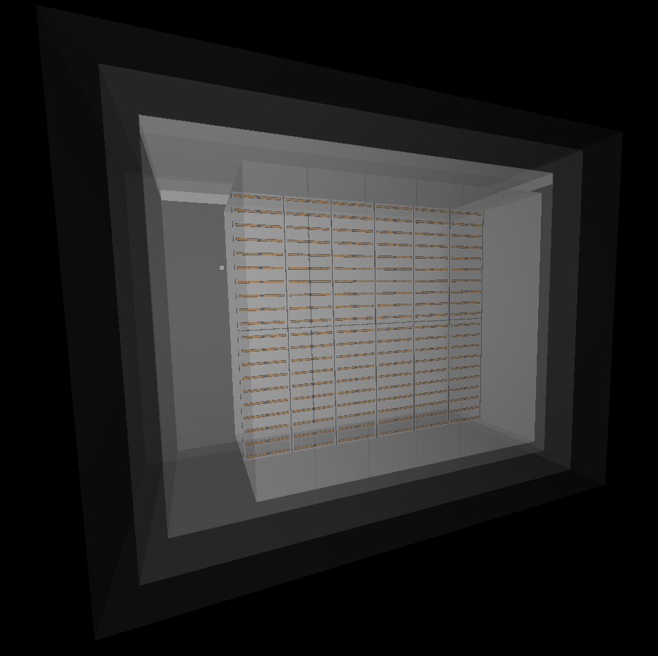
The ‘horizontal drift’ geometry where the ionized charge is pulled towards a wire mesh at the center of the detector. Here the ARAPUCAs are colored orange, and are vertical strips with three sensitive areas inside the wire mesh.
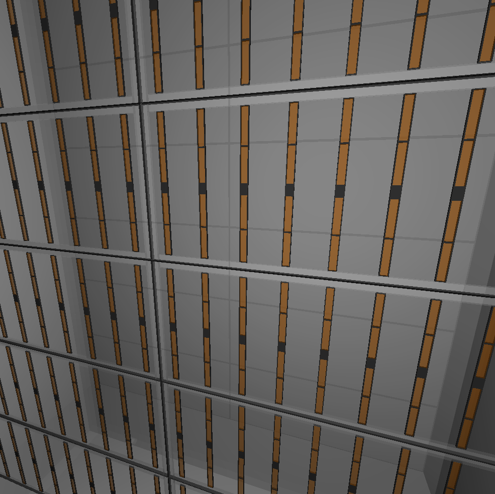
A close-up view of the ARAPUCAs in the ‘horizontal drift’ geometry (rotated 90deg from vertical) with the wire mesh omitted.
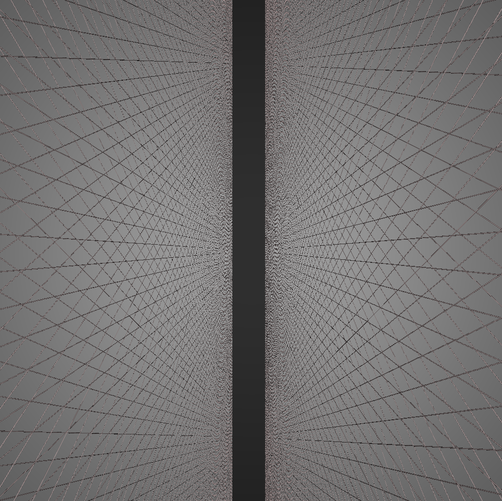
A close-up view of from inside the wire mesh in the ‘horizontal drift’ geometry looking straight at the side of an ARAPUCA. The wire mesh is a few-mm pitch of small wires for collecting ionized charge, and are at three different angles on each side. Physics, not art.
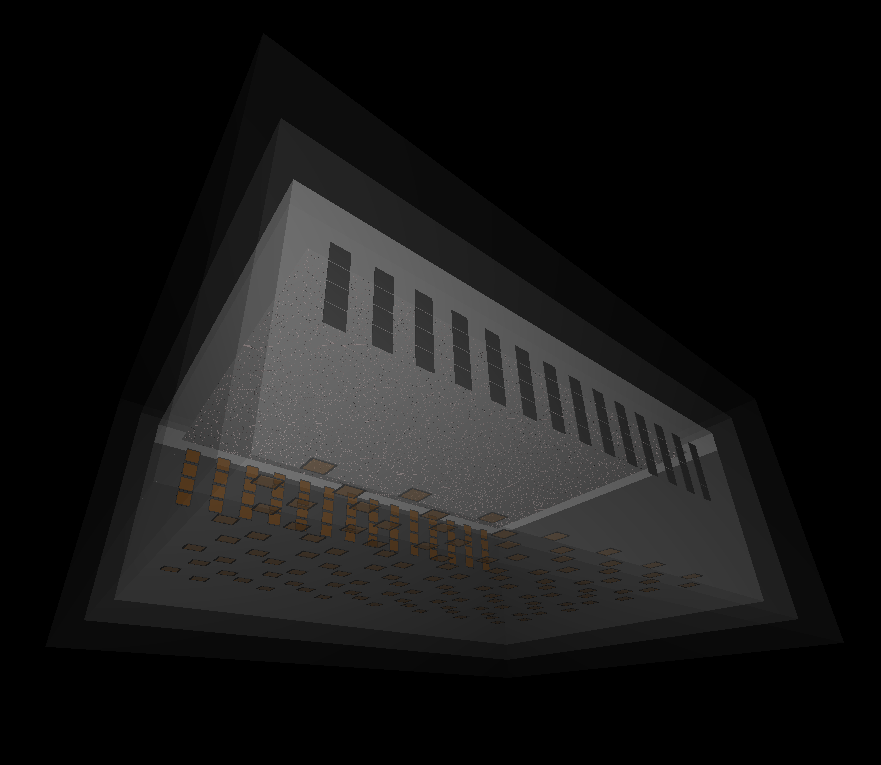
The ‘vertical drift’ geometry where the ionized charge is pulled up strip lines at the top of the detector. Here the ARAPUCAs are colored orange, square tiles placed along two sides and the bottom of the detector.
The following two videos show a visualization of the photons incident on the ARAPUCAs according to the Chroma simulation when 5 MeV electrons are simulated at random locations inside the detector. The electron positions are shown by small red markers, and occasionally high energy gamma rays are produced, which are indicated by green markers. The number of photons incident on each ARAPUCA is visualized by coloring he ARAPUCA with different hues, with red being few and blue being many photons. The detected photons have a clear correlation with the position of the electron, which is part of the information that can be extracted by detecting the light produced in experiments like DUNE.
>> Home