Unbinned maximum likelihood fitting with kernel density estimation

I have previously posted about the basics of maximum likelihood fitting, and how to perform such a fit using binned histograms for both the data and the probability density functions (PDFs). For context, and a gentler introduction to the math, I’d suggest skimming the previous post. In summary, maximum likelihood fitting is a method of statistically determining the makeup of some dataset under the assumption that all possible types of data are described by a finite set of PDFs. Each of the PDFs represent a particular type or class of events in the dataset and describe how the events in that class are distributed along some observable quantities. Observable quantities are things that can be measured for each event, such as energy or position, and different classes of events should have distinct distributions for the maximum likelihood technique to work well. When these PDFs are weighted by a number of events in the class it describes and added together, the resulting distribution can be compared to the total dataset. The correct weighted sum of the PDFs will be maximally similar to the dataset, and an optimization algorithm can be used to find the correct weights.

In this post I will outline an unbinned approach to maximum likelihood fitting and describe kernel density estimation, which is a method of producing unbinned PDFs that are analytically smooth from a finite dataset.

Unbinned maximum likelihood

A binned maximum likelihood fit is computationally efficient and presents minimal bias, as long as the binning is chosen appropriately. Appropriate binning can be difficult, or result in many bins, if the PDFs in the analysis are not smooth or have structure finer than the desired binning. To avoid any bias resulting from binning the PDFs, an unbinned analysis can be performed, which evaluates the PDFs at the exact point of each dataset instead of averaging over the PDF within a bin.

Using the notation similar to the previous post $\mu_k$ is the number of events in event class $k$ where there are $M$ total event classes. Each event class can be described by a normalized PDF $H_k(x_j|\Delta_l)$, which is a function of some set of $j$ observable quantities described by the vector $x_j$. The PDF also depends in principle on some other set of $l$ systematic uncertainties $\Delta_l$. The probability $P(x_j,\Delta_l)$ of observing any particular event described by $x_j$ is therefore $$ P(x_j|\Delta_l) = \frac{1}{\sum_k^M \mu_k} \sum_k^M \mu_k H_k(x_j|\Delta_l) = \frac{1}{\mu} \sum_k^M \mu_k H_k(x_j|\Delta_l) $$ or, in plain English, the weighted average of the probability of each event class. Here, $\mu$ is the sum of all $\mu_k$ events.

A dataset consisting of $N$ event vectors of length $j$ (for the observable quantities) can be written as $x_{ij}$ where $i$ is the event index. The probability of observing this dataset is the product of the probabilities of all $i$ events. $$ P(x_{ij}|\Delta_l) = \prod_i^N P(x_{ij}|\Delta_l) = \mu^{-N} \prod_i^N \sum_k^M \mu_k H_k(x_{ij}|\Delta_l) $$ This probability only accounts for the shape of the distributions, and does not place any constraint on the total number of events. Practically this means that only the ratios $\mu_k/\mu$ are constrained. To constrain the $\mu_k$ parameters directly, include the Poisson probability of observing $N$ events given an expectation of $\mu$ events. $$ \operatorname{Poisson}(N|\mu) = \frac{\mu^N e^{-\mu}}{N!} $$ The total probability, or total likelihood $\mathscr L$, of this dataset is the product of the Poisson probability of observing $N$ events and the likelihood of the events.

$$ {\mathscr L} = \frac{\mu^N e^{-\mu}}{N!} \mu^{-N} \prod_i^N \sum_k^M \mu_k H_k(x_{ij}|\Delta_l) = \frac{e^{-\mu}}{N!} \prod_i^N \sum_k^M \mu_k H_k(x_{ij}|\Delta_l) $$

As before, maximizing the likelihood will be achieved by minimizing the negative logarithm of the likelihood, ${\mathcal L} = -\log {\mathscr L}$, and constant terms that only shift the negative log likelihood are dropped.

$$ {\mathcal L} = \mu - \sum_i^N \log \left( \sum_k^M \mu_k H_k(x_{ij}|\Delta_l) \right) $$

Note that this unbinned likelihood is exactly what one would obtain using a binned likelihood with infinitesimally narrow bins, each containing exactly one datapoint.

The problems with binned PDFs

In principle the binned PDFs created by histogramming events could be used to evaluate the PDFs $H_k$ in an unbinned fit. A significant downside to this method is that it effectively averages over the PDF within each bin, removing any advantage of an unbinned fit. That said, it would technically work as long as datapoints which fell into regions where the PDFs had no events are excluded, as the logarithm of zero is undefined.

Event scarcity and the problem of dimensions

Zero or low probability bins are an even more significant problem for multi-dimensional PDFs than low- or single-dimensional PDFs. To avoid too coarsely binning any dimension, the number of bins tends to grow as a power of the number of dimensions, which means many more simulated events are required to get reasonable statistics in regions of low probability. This often requires extremely large sets of simulated events to get a reasonable binned approximation of a PDF, and if such a simulation effort is not possible, can exclude high-dimensional PDFs as a possibility. A mathematically rigorous way to assign nonzero probability to regions without events would be highly beneficial.

Optimizing systematic parameters

A less obvious downside is present in the treatment of systematic uncertainties $\Delta_l$. These systematics are often treated as transformations to the simulated data that is used to build the PDFs. For instance, a shift or scaling of the observables might be considered, which would account for a potential mismatch between the simulated events used to build PDFs and the actual data events. Either operation would result in events moving between bins, which will result in a discontinuous jump in the likelihood as a systematic parameter is varied. This presents a significant hurdle to gradient descent optimizer algorithms, which often rely on a continuous objective function for convergence. If the optimizer is robust to slight discontinuities, it may still get stuck on local minimums created by the discontinuities.

The simplest solution to this systematic issue is to avoid optimizing the systematic parameters $\Delta_l$ while optimizing the number of events $\mu_k$. Instead, $\mu_k$ is optimized for may sets of fixed values of $\Delta_l$ in an exercise of brute force often called “shift-and-refit.” This effectively maps the likelihood for $\Delta_l$ by profiling the other parameters, and the set with maximum likelihood can be chosen as the best fit. A better solution would allow for the simultaneous optimization of all parameters.

Linearly interpolated PDFs can mitigate the impact of discontinuities to some extent, but generally speaking do not improve

Kernel density estimation

Like binned histograms, kernel density estimation is a method of approximating a PDF from a finite set of data. Unlike binned histograms, kernel density estimation can produce PDFs that are analytically smooth and nonzero at all points. This is done by assigning a distribution (kernel) to each datapoint instead of assuming the datapoint is a delta function at its measured values. There is good motivation for this, as no measurement is infinitely precise. Treating each datapoint as a multi-dimensional Gaussian distribution with widths in each dimension corresponding to the errors of the measurement is therefore quite a reasonable thing to do.

Kernel density estimation (KDE) is quite a bit more general than this, and a one-dimensional KDE PDF with $n$ events with the $i$th event measured at $t_i$ could be written as $$ H_k(x) = \frac{1}{n}\sum_i^n \frac{1}{h_i} K\left(\frac{x-t_i}{h_i}\right) $$ where $K$ is the kernel function and $h_t$ is often called “bandwidth,” but is analogous to the resolution of each measurement. In principle any function $K$ that is normalized $\int K(x)\,dx = 1$ could be used, but sticking with the intuition that the bandwidth is a resolution, a Gaussian is an obvious choice. $$ K(x) = \frac{1}{\sqrt{2 \pi}} e^{-x^2/2} $$ This leads to the following expression for a 1D KDE PDF, which is, as described, a sum of a Gaussian distributions for each datapoint. $$ H_k(x) = \frac{1}{n}\sum_i^n \frac{1}{h_i\sqrt{2 \pi}} e^{-\frac{(x-t_i)^2}{2h_i^2}} $$

Multiple dimensions

With several dimensions in the PDF, totaling $d$ indexed by $j$, the value of each datapoint $i$ is now given by $t_{ij}$ with a matching bandwidth $h_{ij}$. Instead of a single Gaussian, the kernel is now a product of Gaussians, one for each dimension. $$ K(x_j) = \prod_j^d \frac{1}{\sqrt{2 \pi}} e^{-x_j^2/2} $$ Therefore, a multi-dimensional KDE PDF has only a slightly more complicated form than the one-dimensional case. $$ H_k(x_j) = \frac{1}{n}\sum_i^n \prod_j^d \frac{1}{h_{ij}\sqrt{2 \pi}} e^{-\frac{(x_j-t_{ij})^2}{2h_{ij}^2}} $$ This can be simplified from a computational perspective to have fewer exponential evaluations. $$ H_k(x_j) = \frac{1}{n}\sum_i^n \left(h_{ij}\sqrt{2 \pi}\right)^{-d} \exp \left( -\sum_j^d \frac{(x_j-t_{ij})^2}{2h_{ij}^2} \right) $$

Choosing a bandwidth

The bandwidth of each datapoint $i$ in dimension $j$ given by $h_{ij}$ has not yet been determined, except for an intuitive connection that this is related to the resolution of the datapoint. Practically speaking, simply setting the bandwidth to some measurement resolution is not ideal for PDF estimation. The bandwidth effectively represents how much the datapoints are spread out to smooth the distribution. If the bandwidth is too small, individual peaks will be seen for each datapoint, while if it is too large, any input distribution will be smoothed to a Gaussian. It can be shown¹ in one dimension that, for a fixed bandwidth, the optimal choice for bandwidth for a Gaussian kernel is given by $$ h = \left(\frac{1}{2\sqrt{\pi}n\int(P’’(x))^2dx}\right)^{1/5} $$ which has the utterly useless property of depending on the second derivative of the PDF to be estimated: $P’’(x)$. Nevertheless, one can use this to calculate the ideal bandwidth for a known PDF, such as a physicists favorite distribution: a Gaussian with width $\sigma$. $$ h = \left(\frac{4}{3n}\right)^{1/5} \sigma $$ This clearly demonstrates that the ideal bandwidth, roughly speaking, is the width of the distribution to be estimated, and decreases slowly with more events.

For non-Gaussian distributions, this fixed bandwidth will almost always oversmooth the data, and thus poorly approximate the desired PDF. To solve this issue, some fixed-bandwidth method is typically used to produce a first-estimate of the desired PDF $P_0(x)$, and an adaptive bandwidth calculation is done to reduce the smoothing in regions of high probability density. For well-behaved distributions common in particle physics, the following has been proposed² as a method for adaptive calculation of bandwidths. $$h_{ij} = \sigma_j\left(\frac{4}{d+2}\right)^{1/(d+4)}n^{-1/(d+4)}\frac{1}{\sigma (P_0(t_{ij}))^{1/d}} $$ Here, $\sigma = \prod_j^d \sigma_j$ and $P_0$ is some approximation of the PDF to be estimated. This has already made the jump to multiple dimensions, and the number of dimensions $d$ appears several times to correctly account for the geometry in higher dimensions. The terms in this expression can be understood in the following qualitative ways:

• The bandwidth should be proportional to the width in the same dimension $\sigma_j$.
• A factor resulting from the ideal bandwidth estimate for a Gaussian distribution, which is as good a general case as any.
• Reduced bandwidth with more events from inverse proportionality to $n$, where the number of dimensions requires a larger number of events for the same reduction (more smoothing in higher dimensions for same $n$).
• An inverse dependence on $\sigma (P_0(t_{ij}))^{1/d}$, which is roughly the average distance between datapoints in the neighborhood of $t_{ij}$.

Choosing the correct bandwidth is conceptually the hardest part of KDE, but with this general prescription, most PDFs can be well approximated. The accuracy of this approximation should always be checked, either explicitly by comparing to another PDF generation method, or implicitly by testing for bias in the full fit.

Normalization

In the earlier mathematical treatment of an unbinned maximum likelihood fit, the PDFs $H_k(x_j|\Delta_l)$ were assumed to be normalized. The procedure presented to construct KDE PDF does indeed construct a normalized PDF, however it is normalized over the range $(-\infty,+\infty)$. Typically an analysis of data will instead focus on a particular region of the parameter space, either explicitly by setting some boundaries, or implicitly by using parameters without an infinite range, like energy, which must be nonzero. The PDFs used in the analysis must be normalized over the correct range, and the general solution to this is to integrate a PDF over the desired range, and divide future evaluations by this integral.

Fortunately, KDE PDFs with Gaussian kernels as described here can be analytically integrated if the error function is available in a mathematical library. $$ \operatorname{erf} z = \frac{2}{\sqrt{\pi}}\int_0^z e^{-t^2}dt $$ With this, a KDE PDF can be integrated in a region defined by two points $a_j$ and $b_j$. $$ \int_{a_j}^{b_j} H_k(x_j) = \frac{1}{n2^d}\sum_i^n \prod_j^d \left[ \operatorname{erf}\left(\frac{b_j-t_{ij}}{\sqrt{2}h_{ij}}\right) - \operatorname{erf}\left(\frac{a_j-t_{ij}}{\sqrt{2}h_{ij}}\right) \right] $$ While complicated at a glance, this is quite a bit simpler to implement than, for instance, efficiently normalizing (integrating) a linearly interpolated binned PDF.

Handling systematic uncertainties

Finally, systematic uncertainties can be handled by directly transforming the datapoints $t_{ij}$ that go into the PDFs. $$ t_{ij}’ = \operatorname{Syst}(t_{ij},\Delta_j) $$ When systematics are small, this requires no additional calculation besides the data transformation, as each evaluation of the PDF must already consider all datapoints. For large systematics, such as those that significantly modify event weights, the adaptive bandwidth algorithm may need to be rerun. Weights were not explicitly discussed in the previous section, but are trivial to add, as the KDE PDF is an average over the contribution from each datapoint, and this generalizes easily to a weighted average. Assuming each event in the PDF has a weight $w_i$, and the sum of all weights is $w$

$$ H_k(x_j|\Delta_j) = \frac{1}{w}\sum_i^n w_i \left(h_{ij}\sqrt{2 \pi}\right)^{-d} \exp \left( -\sum_j^d \frac{(x_j-t_{ij})^2}{2h_{ij}^2} \right) $$

where the event weights can depend on the systematics or observable values.

Resolution systematics are particularly convenient in the kernel density estimation framework, as they can be directly added in quadrature with the bandwidths. Assuming each dimension includes an additional resolution systematic given by $r_j$, the new bandwidths are given by $$ h_{ij}’ = \sqrt{h_{ij}^2 + r_j^2} $$ In this way all PDF-distorting systematics can be handled in an analytically smooth way.

A computational nightmare

That was a lot of math, both in the potentially-boring sense and the computationally-intensive sense. To give some idea of scale, PDFs for a high-accuracy physics analysis may require $10^4$ - $10^6$ events to achieve sufficient accuracy. Practically, this means to evaluate a KDE PDF as described above at a single point, one must evaluate $10^4$ - $10^6$ exponential functions and associated computations. There will also be many event classes, where $\operatorname{O}(10)$ is a reasonable order of magnitude, tacking another factor of 10 onto the number of exponential functions to evaluate. Even worse, $10^4$ total data events is a lower bound for a physics dataset, meaning the evaluation of the total likelihood is going to need to evaluate each PDF at each of the $10^4$ datapoints.

If you’re keeping track, this means simply computing the total likelihood one time for a physics dataset is going to require $$ 10^4\times10\times10^4 = 10^9 $$ evaluations of the exponential function, minimum, with an upper estimate of $10^{11}$. As I’ve discussed previously evaluating the exponential function is relatively slow, though there are highly optimized routines for this on modern CPUs. For modern CPUs, at least 10 clock cycles, or somewhere between 3 and 10 nanoseconds each would be required. This means optimistically about 3 seconds with an upper estimate of 5 minutes to compute only the exponentials. Considering other calculations that need to be done along with memory bandwidth constraints, the reality is significantly worse than this by a factor of about 100, which leaves us with somewhere between 5 minutes and 8 hours to compute the total likelihood of the data, depending on the size of the dataset and PDF event sample.

The final concern is that any robust optimization algorithm, even with a good seed, is likely going to call its objective function $\operatorname{O}(100)$ times before converging, especially with many optimized parameters. This means a KDE PDF as described is going to take way too long to evaluate on traditional CPU. Of course, this calculation could be paralleled, which on a modern CPU would gain back a factor of 4-8 (or more!), but this is still too long to be feasible. There are approximations that could be made, such as only considering points near-enough to the point of evaluation to contribute significantly, but this is complex in itself. A third option is particularly attractive: utilize the massively parallel computing capabilities of GPUs to perform the calculations.

A modern GPU will have computational abilities in the neighborhood of $10^{12}$ floating-point operations per second (TFLOPs) and incredible memory bandwidth to match. This is achieved with a large fast cache of RAM hooked to several thousand parallel computational cores, each running in parallel. This is exactly the device needed to give worst-case evaluation of the total likelihood in under a minute, and reduce full optimizations to the hour timescale.

A framework for KDE on a GPU

With the framework discussed above, and considering that evaluating KDE PDFs on a CPU will simply take too long, I’ve started work on a kernel density fit framework that uses CUDA kernels to evaluate the PDFs with GPU-acceleration. This is primarily written in Python and uses CuPy to offload math to a GPU. The goal for this framework is to abstract everything necessary to setup an analysis of physics data, binned or unbinned, using either KDE or binned PDFs. Currently, most critical features are implemented.

The framework is organized into kdfit.calculate.Calculation objects which produce some result and depend on other Calculation objects as inputs. A kdfit.calculate.System object manages this collection of calculations and evaluates them as necessary. There are several critical Calculation subclasses:

• kdfit.calculate.Parameter functions as fixed or floated inputs into the calculation, take no Calculation inputs, and can be set programatically.
• kdfit.data.DataLoader contain the code to read data off disk in a way that supports efficient caching. Subclasses are included to read NumPy and HDF5 data.
• kdfit.signal.Signal represents an event class and associated PDF. A Signal takes systematic Parameters and a DataLoader as inputs. There are currently two subclasses that implement different types of PDFs.
  • kdfit.signal.KernelDensityPDF contains the KDE construction and evaluation code for a CPU and GPU
  • kdfit.signal.BinnedPDF contains code to evaluate binned PDFs with and without interpolation, primarily for CPU
• kdfit.observable.Observables represents a multidimensional dataset with configurable dimensions, along with the Signal objects that represent the event classes hypothesized to make up the dataset. Observables accept a DataLoader as input.
• kdfit.term.UnbinnedNegativeLogLikelihoodFunction and kdfit.term.BinnedNegativeLogLikelihoodFunction which take Signal, Observable, and Parameters that scale the Signals as inputs and calculate the likelihood of the Observable data with respect to PDFs derived from the Signal and associated Parameters.

The System and its Calculation objects are setup and managed by a (hopefully) easy to use kdfit.analysis.Analysis interface. The Analysis interface contains the logic to minimize a total negative log likelihood, which can contain one or more sets of Observables and any other terms desired in the likelihood. Eventually pull terms (constraints) will be implemented at this level. Optimization is performed with scipy.optimize.minimize using Parameters that are marked not fixed. Analysis objects also contain logic to find confidence intervals for optimized parameters either by scanning or profiling around a minimum.

Check out the code and see if it is useful for you!

Example analysis

A simple test case using two-dimensional PDFs was used when developing this framework. This contains four signals, A, B, C, and D, which are all two dimensional Gaussians with sigma equal to one on both dimensions, and centered at the four corners of a square (3,3), (3,7), (7,3), (7,7). Data overlaying the generated kernel density PDFs is shown below, where 100 datapoints were used for each PDF.

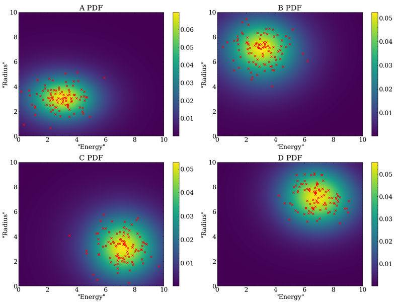
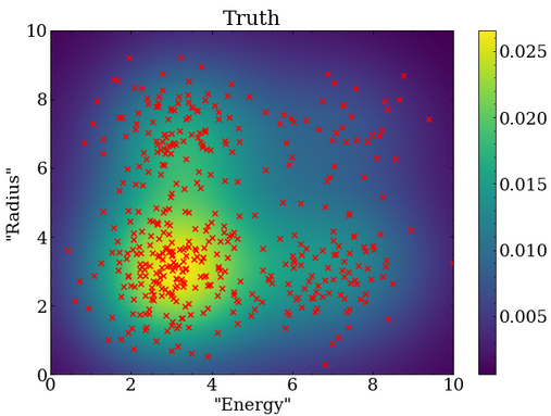
In a real analysis, the number of events in each class would not be known at the start, and instead the optimization algorithm would have to determine them. Since this is a statistical analysis, the optimized results will not be exact, but instead will fluctuate with the exact dataset that is fit. To test that the fitter is working properly, it is common to generate many fake datasets and ensure the distribution of results agree with statistical expectations. 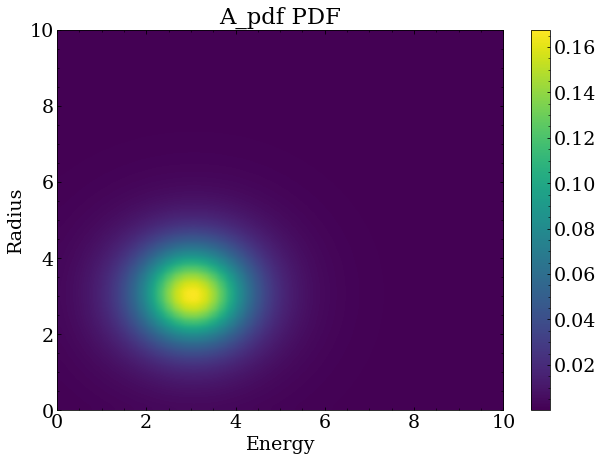For such a test, 250 fake datasets were generated with the Poisson mean event rates described above, and the PDF statistics were greatly increased to $10^5$ events. With this much larger number of events in the PDF, one can see that the shape is noticeably different from the 100 event case shown above.

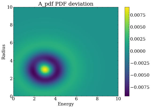
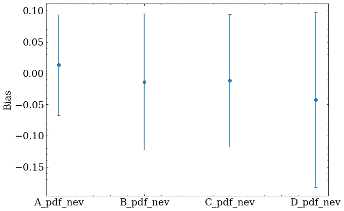
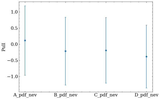
Optimization was repeated for each of the 250 fake datasets, resulting in a set of optimal parameters for each set. Two quantities are useful to obtain for each optimized parameter $x$ with a true value $x_{true}$ and fitted uncertainty $x_{uncert}$.

• Fractional bias given by $(x-x_{true})/x_{true}$
• Pull given by $(x-x_{true})/x_{uncert}$

The offset of the bias and pull from zero shows whether the fitted result is systematically biased in some way. Some bias is expected with approximated PDFs, and should be understood and corrected. Here, the error bars show the width of the bias distribution for each parameter, and the marker shows the mean value from all 250 sets.

Future work

This kdfit package will remain general purpose and open source. I intend to add more features (and possibly radically alter the API!) in the near future, and use this to analyze physics data of my own. A very low bar to reach is some generic ability to add prior constraints to the likelihood calculation, which should be straightfoward. The package also contains the ability to bin both data and PDFs for even faster analyses, which currently use CPU code to do a lot of the heavy lifting, and it would be good to write CUDA kernels for these tasks. When working on an actual analysis, it is also possible (likely!) that a more generic framework for handing systematic parameters will be necessary. Some thought may also go into making this more generally-usable instead of targeted at a physics analysis, but that’s a thought for another day.